{"docs":[{"id":22,"title":"Turning One Reference Spectrum Into Full-Scene Target Detection","slug":"turning-one-reference-spectrum-into-full-scene-target-detection","excerpt":"See how a CNN-based single-spectrum detector trained on Clarity outperformed classical baselines on full-scene MUUFL target detection across multiple train-test scene pairs.","description":"See how a CNN-based single-spectrum detector trained on Clarity outperformed classical baselines on full-scene MUUFL target detection across multiple train-test scene pairs.","type":"Article","author":{"id":7,"name":"Ahmed Sigiuk","slug":"ahmed-sigiuk","email":null,"title":null,"bio":null,"updatedAt":"2026-04-23T23:27:47.142Z","createdAt":"2026-04-23T23:27:47.142Z"},"category":null,"heroImage":{"id":183,"alt":"Turning One Reference Spectrum Into Full-Scene Target Detection","caption":null,"sourcePath":"../src/content/blog/turning-one-reference-spectrum-into-full-scene-target-detection/muufl_gulfport_campus_3.png","updatedAt":"2026-04-23T23:28:03.659Z","createdAt":"2026-04-23T23:28:03.659Z","url":"/api/media/file/muufl_gulfport_campus_3.png","thumbnailURL":"/api/media/file/muufl_gulfport_campus_3-320x305.png","filename":"muufl_gulfport_campus_3.png","mimeType":"image/png","filesize":268373,"width":345,"height":329,"focalX":50,"focalY":50,"sizes":{"thumbnail":{"url":"/api/media/file/muufl_gulfport_campus_3-320x305.png","width":320,"height":305,"mimeType":"image/png","filesize":268415,"filename":"muufl_gulfport_campus_3-320x305.png"},"card":{"url":null,"width":null,"height":null,"mimeType":null,"filesize":null,"filename":null}}},"publishedAt":null,"legacySourcePath":"../src/content/blog/turning-one-reference-spectrum-into-full-scene-target-detection/index.md","bodyMarkdown":"
Using a single reference spectrum per class, a CNN-based detector trained on Clarity outperformed the strongest tested classical baseline in most object-level comparisons on the MUUFL Gulfport dataset (Multi-Unit Spectroscopic Explorer and Hyperspectral Aerial Imagery for Gulfport), an airborne hyperspectral benchmark collected over the University of Southern Mississippi Gulf Park campus in Gulfport, Mississippi.
\n\n\n\n
Introduction
\n\n\n
Hyperspectral target detection is often framed as a practical question: if you know what a target spectrum looks like, can you find that target reliably in airborne imagery? In practice, that is not as simple as matching one clean signature to one clean pixel. The MUUFL Gulfport benchmark contains 64 cloth targets in three sizes; 0.5 m × 0.5 m, 1 m × 1 m, and 3 m × 3 m, while the hyperspectral imagery is delivered at 1 m ground sample distance. That means the benchmark includes targets that are clearly subpixel, targets that are roughly pixel-sized, and targets that span multiple pixels. Many pixels are also mixed pixels, containing not only part of the target signal but also background contributions from nearby vegetation, soil, pavement, rooftops, or other materials. On top of that, the dataset explicitly includes targets that are in shadow or partially or fully occluded by trees, which makes detection even harder.
\n\n\n\n
Classical detectors such as the matched filter (MF), adaptive cosine estimator (ACE), orthogonal subspace projection (OSP), and constrained energy minimization (CEM) remain strong baselines for this type of problem. But an important operational question is whether a learned model can do better when supervision is extremely sparse.
\n\n\n\n
That is what we explored on the MUUFL Gulfport benchmark.
\n\n\n\n
In our setup,each target class is represented by a single reference spectrum, and the task is to detect that target across cross-scene train–test pairs, where the model is trained on one flight image and evaluated on a different flight image. We evaluate three pairs shown in Table 1.. These scene pairs let us test the model across both scene changes and acquisition differences.
\n\n\n\n
Our results focus on four cloth target classes: brown, dark green, pea green, and faux vineyard green. These classes provide a consistent way to compare the learned model against classical baselines across the selected scene pairs.
\n\n\n\n
Train scene
Test scene
Elevation change
Time difference between train and test scene
Campus 1
Campus 3
3500 ft → 3500 ft
~18 hours
Campus 3
Campus 1
3500 ft → 3500 ft
~18 hours
Campus 1
Campus 4
3500 ft → 6700 ft
~47 minutes
Table 1. Train–test scene pairs
\n\n\n\n\n\n\n\n
Property
Value
Bands
72
Wavelengths
367.7 nm to 1043.4 nm
Spatial resolution
1 m GSD
Target classes used here
Brown, dark green, pea green, faux vineyard green
Table 2. MUUFL dataset properties
\n\n\n\n
For this post, we focus on the evaluation view that is most relevant to a real scene-level detection problem: object-level detection quality under low false-alarm constraints. Figures 1 (A, B, and C) gives visual context for the three test scenes emphasized in this post.
We used a CNN spectral model trained on Clarity, Metaspectral’s hyperspectral artificial intelligence platform, for single-spectrum target detection on MUUFL. Here, “single-spectrum” means that each target class is represented by one reference spectrum, which serves as the starting point for model training. On Clarity, the training workflow expands that reference information by generating synthetic target signatures, allowing the detector to learn from a broader set of target-like examples than the original spectrum alone would provide. That matters on MUUFL because the measured image spectra are often not clean target-only signatures. Depending on target size, scene geometry, and local conditions, a pixel may contain a mixture of target and background materials, and the observed target response can also be altered by effects such as shadow or partial tree occlusion.
\n\n\n\n
The model was evaluated against four classical baselines:
\n\n\n\n
MF — matched filter
ACE — adaptive cosine estimator
OSP — orthogonal subspace projection
CEM — constrained energy minimization
\n\n\n\n
For the main result, we use object-level evaluation. Here, the model is judged as an object detector, not just as a pixel scorer. Under the Bullwinkle protocol, the model first produces a dense score map over the scene, and those scores are then converted into object-level detections. Those detections are compared with the known target locations, so performance is measured in terms of whether the detector finds the target objects while avoiding false detections elsewhere in the scene. Figure 2 shows this object-level evaluation for the same campus 1 → 3 dark green case, making the hits, false positives, and missed targets visible in the scene.
\n\n\n\nFigure 2. Object-level scoring overlay for the campus 1 → 3 dark green target case. Green marks hits, red marks false positives, blue marks missed targets, and black marks masked regions.\n\n\n\n
We summarize object-level detection behavior with NAUC (normalized area under the curve). In the Bullwinkle setting, this curve is an operational ROC-style curve that relates probability of detection to false alarms per square meter. Like AUROC, NAUC is threshold-independent: it summarizes performance across all decision thresholds rather than at one fixed threshold. The difference is that AUROC uses the full curve, while NAUC in this study is computed only over the low-false-alarm region up to a cutoff of 0.001 false alarms per square meter. That makes it especially useful when false positives matter, since it rewards detectors that stay strong in the operating region most relevant for practical target detection. Figure 3 shows one example of this curve for the campus 1 → 3 dark green case.
\n\n\n\nFigure 3. Object-level detection curve for the campus 1 → 3 dark green target case. The Bullwinkle curve plots probability of detection against false alarms per square meter, with NAUC computed up to the 0.001 cutoff.\n\n\n\n
The workflow was run on Clarity end to end: hyperspectral data can be uploaded, labeled, used to train and evaluate models, and then carried forward into deployment-oriented target-detection workflows. That broader workflow is part of what makes these results meaningful beyond a single benchmark run. It makes benchmark results easier to reproduce, methods easier to compare under a consistent setup, and successful models easier to move toward deployment.
\n\n\n\n
Figure 4 shows the CNN score maps before object-level post-processing or metric evaluation. Each panel corresponds to one target class and one train–test scene pair, with brighter regions indicating stronger target likelihood. These maps are useful because they show not just where the model responds, but how concentrated or diffuse those responses are across the scene. In turn, that helps explain why some class/scene combinations translate into cleaner object-level detections than others.
\n\n\n\n
campus 1 → campus 3
campus 3 → campus 1
campus 1 → campus 4
Dark Green
Brown
Pea Green
Faux vineyard green
Figure 4. Example raw prediction map from the CNN model.
\n\n\n\n
Key Findings
\n\n\n\n
The strongest result in this study comes from the object-level evaluation described above, where the model is judged on whether its scene-level detections recover target objects while avoiding false alarms elsewhere in the image. We summarize that behavior with object-level NAUC, a normalized 0-to-1 score in which higher values indicate better low-false-alarm detection performance. Table 3 summarizes the overall outcome across all train–test scene pairs, while Table 4 (A, B and C) provides the class-by-class breakdown for each pair. Under this object-level measure, the CNN outperformed the best tested classical baseline in 9 of 12 comparisons. Here, the classical comparison is not tied to one fixed method; for each case, it refers to whichever of MF, ACE, OSP, or CEM performed best.
\n\n\n\n
Train–Test scene pair
NAUC wins
campus 1 → 3
4 / 4
campus 3 → 1
3 / 4
campus 1 → 4
2 / 4
Overall
9 / 12
Table 3. Object-level summary across train–test scene pairs
\n\n\n\n
Object-level results by train–test scene pair
\n\n\n\n
The scene-pair comparisons make it easier to see how performance changes from one train–test setup to another.
\n\n\n\n
Class
CNN NAUC
Best classical
Classical NAUC
Δ
Dark green
0.442
MF
0.386
+0.056
Brown
0.512
MF
0.432
+0.080
Pea green
0.310
MF
0.294
+0.016
Faux vineyard green
0.564
CEM
0.428
+0.136
Table 4A. Object-level comparison for campus 1 → 3
\n\n\n\n
In Table 4A, campus 1 → 3 train-test scene pair, the CNN is ahead in all four classes. This is the strongest and cleanest transfer result in the set.
\n\n\n\n
Class
CNN NAUC
Best classical
Classical NAUC
Δ
Dark green
0.444
ACE
0.423
+0.021
Brown
0.715
ACE
0.665
+0.050
Pea green
0.382
MF
0.435
-0.053
Faux vineyard green
0.662
ACE
0.613
+0.049
Table 4B. Object-level comparison for campus 3 → 1
\n\n\n\n
In Table 4B, campus 3 → 1 train-test scene pair the same pattern largely holds: the CNN remains ahead in three of the four classes.
\n\n\n\n
Class
CNN NAUC
Best classical
Classical NAUC
Δ
Dark green
0.401
MF
0.311
+0.090
Brown
0.595
MF
0.561
+0.034
Pea green
0.272
MF
0.310
-0.038
Faux vineyard green
0.408
MF
0.432
-0.024
Table 4C. Object-level comparison for campus 1 → 4
\n\n\n\n
In Table 4C, the campus 1 → 4 train–test scene pair is the toughest of the three because it introduces the largest scene and acquisition change, including a shift from the 3500 ft collection group to the 6700 ft group. This makes it the most distinct train–test pairing in the study and provides a likely explanation for the lower CNN performance: in a single-spectrum setting, larger differences in scene and acquisition conditions can make the observed target spectra less consistent with the training signatures, which in turn makes detection harder.
\n\n\n\n
Discussion
\n\n\n\n
The most important point in these results is not simply that a CNN outperformed several classical baselines.
\n\n\n\n
The more useful point is how little information the model needed to get there.
\n\n\n\n
This was a single-spectrum setup: one reference spectrum per class, applied across cross-flight train–test scene pairs. That lowers the barrier to building practical target-detection workflows. In many real Earth observation (EO) settings, assembling large, carefully curated target datasets is expensive or unrealistic. A workflow that can begin from a single target spectrum is therefore operationally attractive.
\n\n\n\n
That is where the platform angle becomes important. The value here is not only the CNN itself, but the full workflow that turns a single reference spectrum into an operational target-detection pipeline. On Clarity, that starts by expanding the reference spectrum into synthetic target signatures for training. This helps because a single measured spectrum does not fully represent how a target will appear in real airborne imagery, where the observed signal can shift because of mixing, illumination, shadow, and surrounding materials. By exposing the model to a broader set of target-like examples, the workflow makes training more robust than relying on the original spectrum alone. From there, the same platform supports data upload, labeling, model training, evaluation, and deployment, making the results easier to reproduce and the path to operational use much more direct.
\n\n\n\n
The results also highlight an important point about how target-detection systems should be evaluated. For this study, object-level evaluation is the most relevant measure because the task is to find target objects across the scene under false-alarm constraints. In other applications, pixel-level evaluation may be more appropriate, particularly when the emphasis is on pixel-wise target separation rather than full-scene object detection.
\n\n\n\n
Conclusion
\n\n\n\n
On the MUUFL Gulfport benchmark, a CNN single-spectrum detector trained on Clarity outperformed a family of classical baselines in most object-level comparisons across multiple cross-flight train–test scene pairs.
\n\n\n\n
More importantly, these results show that practical hyperspectral target detection does not always require large target datasets or complex supervision. A single reference spectrum can be enough to drive a strong detection workflow when combined with a learned model and a platform that supports the full process from data ingestion through evaluation and deployment.
\n\n\n\n
That is the broader takeaway from this study: the value is not only in the model, but in the ability to turn a single-spectrum detection problem into a repeatable, operational workflow.
\n","bodyHtml":"
Using a single reference spectrum per class, a CNN-based detector trained on Clarity outperformed the strongest tested classical baseline in most object-level comparisons on the MUUFL Gulfport dataset (Multi-Unit Spectroscopic Explorer and Hyperspectral Aerial Imagery for Gulfport), an airborne hyperspectral benchmark collected over the University of Southern Mississippi Gulf Park campus in Gulfport, Mississippi.
\n
Introduction
\n\n
Hyperspectral target detection is often framed as a practical question: if you know what a target spectrum looks like, can you find that target reliably in airborne imagery? In practice, that is not as simple as matching one clean signature to one clean pixel. The MUUFL Gulfport benchmark contains 64 cloth targets in three sizes; 0.5 m × 0.5 m, 1 m × 1 m, and 3 m × 3 m, while the hyperspectral imagery is delivered at 1 m ground sample distance. That means the benchmark includes targets that are clearly subpixel, targets that are roughly pixel-sized, and targets that span multiple pixels. Many pixels are also mixed pixels, containing not only part of the target signal but also background contributions from nearby vegetation, soil, pavement, rooftops, or other materials. On top of that, the dataset explicitly includes targets that are in shadow or partially or fully occluded by trees, which makes detection even harder.
\n
Classical detectors such as the matched filter (MF), adaptive cosine estimator (ACE), orthogonal subspace projection (OSP), and constrained energy minimization (CEM) remain strong baselines for this type of problem. But an important operational question is whether a learned model can do better when supervision is extremely sparse.
\n
That is what we explored on the MUUFL Gulfport benchmark.
\n
In our setup,each target class is represented by a single reference spectrum, and the task is to detect that target across cross-scene train–test pairs, where the model is trained on one flight image and evaluated on a different flight image. We evaluate three pairs shown in Table 1.. These scene pairs let us test the model across both scene changes and acquisition differences.
\n
Our results focus on four cloth target classes: brown, dark green, pea green, and faux vineyard green. These classes provide a consistent way to compare the learned model against classical baselines across the selected scene pairs.
\n
Train scene
Test scene
Elevation change
Time difference between train and test scene
Campus 1
Campus 3
3500 ft → 3500 ft
~18 hours
Campus 3
Campus 1
3500 ft → 3500 ft
~18 hours
Campus 1
Campus 4
3500 ft → 6700 ft
~47 minutes
Table 1. Train–test scene pairs
\n\n
Property
Value
Bands
72
Wavelengths
367.7 nm to 1043.4 nm
Spatial resolution
1 m GSD
Target classes used here
Brown, dark green, pea green, faux vineyard green
Table 2. MUUFL dataset properties
\n
For this post, we focus on the evaluation view that is most relevant to a real scene-level detection problem: object-level detection quality under low false-alarm constraints. Figures 1 (A, B, and C) gives visual context for the three test scenes emphasized in this post.
\n
\n
\n
\n
\nFigure 1A. Campus 1\n
\n
\n
\n
\nFigure 1B. Campus 3\n\nFigure 1C.Campus 4\n
Approach
\n
We used a CNN spectral model trained on Clarity, Metaspectral’s hyperspectral artificial intelligence platform, for single-spectrum target detection on MUUFL. Here, “single-spectrum” means that each target class is represented by one reference spectrum, which serves as the starting point for model training. On Clarity, the training workflow expands that reference information by generating synthetic target signatures, allowing the detector to learn from a broader set of target-like examples than the original spectrum alone would provide. That matters on MUUFL because the measured image spectra are often not clean target-only signatures. Depending on target size, scene geometry, and local conditions, a pixel may contain a mixture of target and background materials, and the observed target response can also be altered by effects such as shadow or partial tree occlusion.
\n
The model was evaluated against four classical baselines:
\n
MF — matched filter
ACE — adaptive cosine estimator
OSP — orthogonal subspace projection
CEM — constrained energy minimization
\n
For the main result, we use object-level evaluation. Here, the model is judged as an object detector, not just as a pixel scorer. Under the Bullwinkle protocol, the model first produces a dense score map over the scene, and those scores are then converted into object-level detections. Those detections are compared with the known target locations, so performance is measured in terms of whether the detector finds the target objects while avoiding false detections elsewhere in the scene. Figure 2 shows this object-level evaluation for the same campus 1 → 3 dark green case, making the hits, false positives, and missed targets visible in the scene.
\nFigure 2. Object-level scoring overlay for the campus 1 → 3 dark green target case. Green marks hits, red marks false positives, blue marks missed targets, and black marks masked regions.\n
We summarize object-level detection behavior with NAUC (normalized area under the curve). In the Bullwinkle setting, this curve is an operational ROC-style curve that relates probability of detection to false alarms per square meter. Like AUROC, NAUC is threshold-independent: it summarizes performance across all decision thresholds rather than at one fixed threshold. The difference is that AUROC uses the full curve, while NAUC in this study is computed only over the low-false-alarm region up to a cutoff of 0.001 false alarms per square meter. That makes it especially useful when false positives matter, since it rewards detectors that stay strong in the operating region most relevant for practical target detection. Figure 3 shows one example of this curve for the campus 1 → 3 dark green case.
\nFigure 3. Object-level detection curve for the campus 1 → 3 dark green target case. The Bullwinkle curve plots probability of detection against false alarms per square meter, with NAUC computed up to the 0.001 cutoff.\n
The workflow was run on Clarity end to end: hyperspectral data can be uploaded, labeled, used to train and evaluate models, and then carried forward into deployment-oriented target-detection workflows. That broader workflow is part of what makes these results meaningful beyond a single benchmark run. It makes benchmark results easier to reproduce, methods easier to compare under a consistent setup, and successful models easier to move toward deployment.
\n
Figure 4 shows the CNN score maps before object-level post-processing or metric evaluation. Each panel corresponds to one target class and one train–test scene pair, with brighter regions indicating stronger target likelihood. These maps are useful because they show not just where the model responds, but how concentrated or diffuse those responses are across the scene. In turn, that helps explain why some class/scene combinations translate into cleaner object-level detections than others.
\n
campus 1 → campus 3
campus 3 → campus 1
campus 1 → campus 4
Dark Green
Brown
Pea Green
Faux vineyard green
Figure 4. Example raw prediction map from the CNN model.
\n
Key Findings
\n
The strongest result in this study comes from the object-level evaluation described above, where the model is judged on whether its scene-level detections recover target objects while avoiding false alarms elsewhere in the image. We summarize that behavior with object-level NAUC, a normalized 0-to-1 score in which higher values indicate better low-false-alarm detection performance. Table 3 summarizes the overall outcome across all train–test scene pairs, while Table 4 (A, B and C) provides the class-by-class breakdown for each pair. Under this object-level measure, the CNN outperformed the best tested classical baseline in 9 of 12 comparisons. Here, the classical comparison is not tied to one fixed method; for each case, it refers to whichever of MF, ACE, OSP, or CEM performed best.
\n
Train–Test scene pair
NAUC wins
campus 1 → 3
4 / 4
campus 3 → 1
3 / 4
campus 1 → 4
2 / 4
Overall
9 / 12
Table 3. Object-level summary across train–test scene pairs
\n
Object-level results by train–test scene pair
\n
The scene-pair comparisons make it easier to see how performance changes from one train–test setup to another.
\n
Class
CNN NAUC
Best classical
Classical NAUC
Δ
Dark green
0.442
MF
0.386
+0.056
Brown
0.512
MF
0.432
+0.080
Pea green
0.310
MF
0.294
+0.016
Faux vineyard green
0.564
CEM
0.428
+0.136
Table 4A. Object-level comparison for campus 1 → 3
\n
In Table 4A, campus 1 → 3 train-test scene pair, the CNN is ahead in all four classes. This is the strongest and cleanest transfer result in the set.
\n
Class
CNN NAUC
Best classical
Classical NAUC
Δ
Dark green
0.444
ACE
0.423
+0.021
Brown
0.715
ACE
0.665
+0.050
Pea green
0.382
MF
0.435
-0.053
Faux vineyard green
0.662
ACE
0.613
+0.049
Table 4B. Object-level comparison for campus 3 → 1
\n
In Table 4B, campus 3 → 1 train-test scene pair the same pattern largely holds: the CNN remains ahead in three of the four classes.
\n
Class
CNN NAUC
Best classical
Classical NAUC
Δ
Dark green
0.401
MF
0.311
+0.090
Brown
0.595
MF
0.561
+0.034
Pea green
0.272
MF
0.310
-0.038
Faux vineyard green
0.408
MF
0.432
-0.024
Table 4C. Object-level comparison for campus 1 → 4
\n
In Table 4C, the campus 1 → 4 train–test scene pair is the toughest of the three because it introduces the largest scene and acquisition change, including a shift from the 3500 ft collection group to the 6700 ft group. This makes it the most distinct train–test pairing in the study and provides a likely explanation for the lower CNN performance: in a single-spectrum setting, larger differences in scene and acquisition conditions can make the observed target spectra less consistent with the training signatures, which in turn makes detection harder.
\n
Discussion
\n
The most important point in these results is not simply that a CNN outperformed several classical baselines.
\n
The more useful point is how little information the model needed to get there.
\n
This was a single-spectrum setup: one reference spectrum per class, applied across cross-flight train–test scene pairs. That lowers the barrier to building practical target-detection workflows. In many real Earth observation (EO) settings, assembling large, carefully curated target datasets is expensive or unrealistic. A workflow that can begin from a single target spectrum is therefore operationally attractive.
\n
That is where the platform angle becomes important. The value here is not only the CNN itself, but the full workflow that turns a single reference spectrum into an operational target-detection pipeline. On Clarity, that starts by expanding the reference spectrum into synthetic target signatures for training. This helps because a single measured spectrum does not fully represent how a target will appear in real airborne imagery, where the observed signal can shift because of mixing, illumination, shadow, and surrounding materials. By exposing the model to a broader set of target-like examples, the workflow makes training more robust than relying on the original spectrum alone. From there, the same platform supports data upload, labeling, model training, evaluation, and deployment, making the results easier to reproduce and the path to operational use much more direct.
\n
The results also highlight an important point about how target-detection systems should be evaluated. For this study, object-level evaluation is the most relevant measure because the task is to find target objects across the scene under false-alarm constraints. In other applications, pixel-level evaluation may be more appropriate, particularly when the emphasis is on pixel-wise target separation rather than full-scene object detection.
\n
Conclusion
\n
On the MUUFL Gulfport benchmark, a CNN single-spectrum detector trained on Clarity outperformed a family of classical baselines in most object-level comparisons across multiple cross-flight train–test scene pairs.
\n
More importantly, these results show that practical hyperspectral target detection does not always require large target datasets or complex supervision. A single reference spectrum can be enough to drive a strong detection workflow when combined with a learned model and a platform that supports the full process from data ingestion through evaluation and deployment.
\n
That is the broader takeaway from this study: the value is not only in the model, but in the ability to turn a single-spectrum detection problem into a repeatable, operational workflow.
","updatedAt":"2026-04-28T15:19:03.734Z","createdAt":"2026-04-23T23:28:04.113Z","_status":"published"},{"id":21,"title":"Lithium Detection over the McDermitt Deposit Using Metaspectral’s Clarity Platform","slug":"lithium-detection-hyperspectral-imaging-metaspectral","excerpt":"Lithium detection pipeline at the McDermitt deposit using EnMAP hyperspectral data and Metaspectral’s Clarity analysis platform.","description":"Lithium detection pipeline at the McDermitt deposit using EnMAP hyperspectral data and Metaspectral’s Clarity analysis platform.","type":"Article","author":{"id":6,"name":"Guillaume Hans","slug":"guillaume-hans","email":null,"title":null,"bio":null,"updatedAt":"2026-04-23T23:27:03.623Z","createdAt":"2026-04-23T23:27:03.623Z"},"category":null,"heroImage":{"id":133,"alt":"Lithium Detection over the McDermitt Deposit Using Metaspectral’s Clarity Platform","caption":null,"sourcePath":"../src/content/blog/lithium-detection-hyperspectral-imaging-metaspectral/feature_img.jpg","updatedAt":"2026-04-23T23:27:16.043Z","createdAt":"2026-04-23T23:27:16.043Z","url":"/api/media/file/feature_img.jpg","thumbnailURL":"/api/media/file/feature_img-320x149.jpg","filename":"feature_img.jpg","mimeType":"image/jpeg","filesize":562960,"width":1916,"height":892,"focalX":50,"focalY":50,"sizes":{"thumbnail":{"url":"/api/media/file/feature_img-320x149.jpg","width":320,"height":149,"mimeType":"image/jpeg","filesize":14951,"filename":"feature_img-320x149.jpg"},"card":{"url":"/api/media/file/feature_img-768x358.jpg","width":768,"height":358,"mimeType":"image/jpeg","filesize":77505,"filename":"feature_img-768x358.jpg"}}},"publishedAt":"2026-04-16T01:28:48.000Z","legacySourcePath":"../src/content/blog/lithium-detection-hyperspectral-imaging-metaspectral/index.md","bodyMarkdown":"
The global race for critical minerals is putting pressure on traditional exploration methods. The hunt for “white gold”, lithium, is shifting from traditional soil sampling toward advanced hyperspectral imaging to identify resources that are too remote or complex. Accelerating this discovery is vital for the green energy transition, but it requires tools that can process massive satellite datasets with geological precision.
\n\n\n\n
A landmark study by Asadzadeh & Chabrillat (2025) demonstrates this potential in the McDermitt Caldera, the largest known lithium deposit in the United States, located in south-east Oregon at the Nevada border. Their research utilizes EnMAP satellite data and a methodology called “Mixture-Tuned Feature Matching” (MTFM) to accurately detect lithium-bearing minerals. MTFM works by isolating diagnostic absorption features through continuum removal, generating synthetic library mixtures at discrete increments, and performing least-square fitting to find the best spectral match for every image pixel.
\n\n\n\n
Metaspectral’s Clarity Platform is designed to bring this level of academic rigor to the industrial scale. As a high-performance, cloud-native hyperspectral analysis platform, Clarity allows exploration teams to replicate this type of workflow while comparing it against Clarity’s internal deep learning tools. In this post, we walk through the replication of the MTFM lithium detection pipeline, from initial unmixing to sub-nanometer polynomial fitting, and show how AI-driven target detection can be used to rapidly identify high-potential zones before performing detailed spectral analysis.
\n\n\n\n
Leveraging EnMAP Imagery
\n\n\n\n
For this study, like Asadzadeh & Chabrillat (2025), we utilize data from the Environmental Mapping and Analysis Program (EnMAP). EnMAP provides high-quality hyperspectral data with 242 bands across the visible and near-infrared (VNIR) and short-wave infrared (SWIR) regions (420 nm to 2450 nm). Its spectral sampling of approximately 6.5 nm in the VNIR and 10 nm in the SWIR makes it uniquely suited for mineral exploration. Clarity is designed to directly ingest EnMAP’s products, allowing us to focus directly on our task: lithium detection. Figure 1 shows the EnMAP image acquired over the McDermitt deposit.
\n\n\n\nFigure 1: EnMAP image acquired over the McDermitt deposit (OR & NV, USA), acquired on June 22nd 2024.\n\n\n\n
Lithium detection workflow in Clarity
\n\n\n\n
Lithium in the McDermitt deposit is primarily hosted in Hectorite, a lithium-rich smectite clay. The key to identifying it remotely lies in the SWIR spectrum, specifically the 2200–2400 nm region. This range contains diagnostic absorption features for lithium-bearing clays, which shift slightly depending on the substitution of Lithium (Li) for Magnesium (Mg) in the mineral lattice.
\n\n\n\n
To translate these geological markers into a digital map, we leverage the following workflow within the Clarity environment.
\n\n\n\n
Vegetation masking
\n\n\n\n
Before looking for minerals, we must remove “noise” from the landscape. In areas with sparse or dense vegetation, Photosynthetic Vegetation (PV) and Non-Photosynthetic Vegetation (NPV) can obscure mineral signatures. Using Clarity’s Linear Spectral Unmixing tool, we decompose each pixel into Soil, PV, and NPV components. This results in abundance maps shown in Figure 2, corresponding to each of these endmembers. All pixels from the ENMAP image for which the Soil fraction was smaller than 0.5 (50%) were masked.
\n\n\n\nFigure 2: Fractions (abundances) of Soil, Photosynthetic Vegetation (PV) and Non-Photosynthetic Vegetation (NPV).\n\n\n\n
Continuum Removal for Feature Enhancement
\n\n\n\n
To compare mineral signatures accurately, we must isolate the absorption pits from the overall “slope” of the reflectance curve. This is achieved through Continuum Removal (CR).
\n\n\n\n
In raw spectra, the true shape of an absorption feature is often distorted by the background reflectance (“continuum”) caused by factors like grain size, surface moisture, or other non-target minerals. This background creates an overall slope that can shift the apparent position of an absorption minimum or make a deep feature appear shallow. By removing this continuum, we effectively “zoom in” on the chemical bonds of the mineral itself, effectively normalizing the data so that the depth and shape of the Hectorite absorption feature become the primary variables (as illustrated in Figure 3).
\n\n\n\n
In Clarity, CR is achieved using a fast convex hull computation algorithm. This process “flattens” the spectrum between 2200 and 2400 nm, allowing for precise comparison between image pixels and library standards.
\n\n\n\nFigure 3: USGS reflectance spectra of Hectorite, Nontronite and Saponite before and after continuum removal.\n\n\n\n
Library Spectra and Synthetic Mixtures
\n\n\n\n
The ENMAP image spectra are compared against gold-standard spectra from the USGS library. Following Asadzadeh & Chabrillat (2025), spectra from three minerals were selected: Hectorite, Nontronite, and Saponite. Indeed, while Hectorite is the primary lithium-bearing mineral at McDermitt, it rarely occurs in isolation. It is typically found within a complex assemblage of smectite clays, including Nontronite (Fe-rich) and Saponite (Mg-rich). Identifying the specific “sweet spot” of lithium mineralization requires distinguishing Hectorite from these spectrally similar neighbors (Figure 3). To account for this, Clarity generates linear mixtures of these three primary minerals based on their spectra, automatically resamples them to match the specific wavelength intervals of ENMAP and applies the same CR pre-processing. This provides a comprehensive reference set for the complex mineralogies found at the McDermitt site (Figure 4).
\n\n\n\nFigure 4:Hectorite – Nontronite – Saponite spectral mixtures representing the complex mineralogies found at the McDermitt site.\n\n\n\n
Mixture Tuned Feature Matching (MTFM)
\n\n\n\n
This is the “engine room” of this lithium detection approach. MTFM performs a Least Square Fitting to match each image pixel against every synthetic mixture presented above (Figure 4) and computes the Pearson Correlation. The specific mixture that yielded the highest match is retained along with the correlation value. To maximize the signal-to-noise ratio and ensure high-confidence detections, we retain only pixels with a correlation higher than 90%. This procedure provides a robust estimate of mineral presence. The correlation value serves as a proxy for mineral abundance, allowing us to generate a heatmap ranging from low to high lithium potential. These heatmaps are presented in Figure 5 where pixels with a correlation lower than 90% were masked for visual interpretability purposes.
\n\n\n\nFigure 5: Heatmap of Pearson Correlation along with Hectorite, Nontronite and Saponite abundance as defined in the synthetic spectra mixtures. Pixels with correlation smaller then 0.9 were masked for clarity purposes.\n\n\n\n
Streamlining the Workflow with Deep Learning
\n\n\n\n
While the MTFM approach is highly effective, the preprocessing required, the manual creation of synthetic mixtures and iterative least-square fitting can be computationally intensive and time-consuming. To accelerate discovery, Clarity offers a Deep Learning Target Detection model.
\n\n\n\n
By using the USGS Hectorite spectrum directly as a target, the deep learning model can generate an abundance map (Figure 6) that rivals the accuracy of the MTFM approach while bypassing the preprocessing, mixture creation, and fitting stages entirely. This reduces the time and effort required, thereby offering potential for rapid field deployment and decision-making.
\n\n\n\nFigure 6: Hectorite abundance derived using Clarity’s deep learning-based target detection method.\n\n\n\n
Hectorite Lithium Richness
\n\n\n\n
The final and most precise step involves finding the analytic minimum of the hectorite absorption pit. This analysis can be applied directly to the high-confidence pixels identified via the MTFM workflow or the Deep Learning model. Because lithium content causes a subtle shift in the position of the absorption pit, a 4th-order polynomial is fitted to the pixels with the highest hectorite abundance. Despite EnMAP’s 10 nm spectral sampling, polynomial fitting allows Clarity to estimate the exact wavelength of the minimum at a sub-nanometer scale. By mapping these precise wavelength positions across the deposit (Figure 7), Clarity effectively grades the lithium concentration of the Hectorite clays from space or aircraft. Higher Lithium content is translated by a shift of the absorption pit towards lower wavelengths.
\n\n\n\nFigure 7: Hectorite composition in terms of Lithium versus Magnesium content. \n\n\n\n
Conclusion
\n\n\n\n
Metaspectral’s Clarity platform moves your hyperspectral data from reflectance to actionable mineralogical maps. Clarity provides the flexibility to compare and combine industry-standard methodologies with modern AI-driven tools to replicate and scale state-of-the-art research. This dual-pathway approach ensures both operational efficiency and geological accuracy, securing the future of the global critical minerals and green energy sectors.
\n\n\n\n
Are you exploring Lithium or other critical minerals?
\n\n\n\n
Contact Metaspectral to see how Clarity can accelerate your discovery timelines.
\n\n\n\n\n\n\n\n
References
\n\n\n\n
Asadzadeh, S. & Chabrillat, S. (2025). Leveraging EnMAP hyperspectral data for mineral exploration: Examples from different deposit types. Ore Geology Reviews, 186, 106912. https://doi.org/10.1016/j.oregeorev.2025.106912
","bodyHtml":"
The global race for critical minerals is putting pressure on traditional exploration methods. The hunt for “white gold”, lithium, is shifting from traditional soil sampling toward advanced hyperspectral imaging to identify resources that are too remote or complex. Accelerating this discovery is vital for the green energy transition, but it requires tools that can process massive satellite datasets with geological precision.
\n
A landmark study by Asadzadeh & Chabrillat (2025) demonstrates this potential in the McDermitt Caldera, the largest known lithium deposit in the United States, located in south-east Oregon at the Nevada border. Their research utilizes EnMAP satellite data and a methodology called “Mixture-Tuned Feature Matching” (MTFM) to accurately detect lithium-bearing minerals. MTFM works by isolating diagnostic absorption features through continuum removal, generating synthetic library mixtures at discrete increments, and performing least-square fitting to find the best spectral match for every image pixel.
\n
Metaspectral’s Clarity Platform is designed to bring this level of academic rigor to the industrial scale. As a high-performance, cloud-native hyperspectral analysis platform, Clarity allows exploration teams to replicate this type of workflow while comparing it against Clarity’s internal deep learning tools. In this post, we walk through the replication of the MTFM lithium detection pipeline, from initial unmixing to sub-nanometer polynomial fitting, and show how AI-driven target detection can be used to rapidly identify high-potential zones before performing detailed spectral analysis.
\n
Leveraging EnMAP Imagery
\n
For this study, like Asadzadeh & Chabrillat (2025), we utilize data from the Environmental Mapping and Analysis Program (EnMAP). EnMAP provides high-quality hyperspectral data with 242 bands across the visible and near-infrared (VNIR) and short-wave infrared (SWIR) regions (420 nm to 2450 nm). Its spectral sampling of approximately 6.5 nm in the VNIR and 10 nm in the SWIR makes it uniquely suited for mineral exploration. Clarity is designed to directly ingest EnMAP’s products, allowing us to focus directly on our task: lithium detection. Figure 1 shows the EnMAP image acquired over the McDermitt deposit.
\nFigure 1: EnMAP image acquired over the McDermitt deposit (OR & NV, USA), acquired on June 22nd 2024.\n
Lithium detection workflow in Clarity
\n
Lithium in the McDermitt deposit is primarily hosted in Hectorite, a lithium-rich smectite clay. The key to identifying it remotely lies in the SWIR spectrum, specifically the 2200–2400 nm region. This range contains diagnostic absorption features for lithium-bearing clays, which shift slightly depending on the substitution of Lithium (Li) for Magnesium (Mg) in the mineral lattice.
\n
To translate these geological markers into a digital map, we leverage the following workflow within the Clarity environment.
\n
Vegetation masking
\n
Before looking for minerals, we must remove “noise” from the landscape. In areas with sparse or dense vegetation, Photosynthetic Vegetation (PV) and Non-Photosynthetic Vegetation (NPV) can obscure mineral signatures. Using Clarity’s Linear Spectral Unmixing tool, we decompose each pixel into Soil, PV, and NPV components. This results in abundance maps shown in Figure 2, corresponding to each of these endmembers. All pixels from the ENMAP image for which the Soil fraction was smaller than 0.5 (50%) were masked.
\nFigure 2: Fractions (abundances) of Soil, Photosynthetic Vegetation (PV) and Non-Photosynthetic Vegetation (NPV).\n
Continuum Removal for Feature Enhancement
\n
To compare mineral signatures accurately, we must isolate the absorption pits from the overall “slope” of the reflectance curve. This is achieved through Continuum Removal (CR).
\n
In raw spectra, the true shape of an absorption feature is often distorted by the background reflectance (“continuum”) caused by factors like grain size, surface moisture, or other non-target minerals. This background creates an overall slope that can shift the apparent position of an absorption minimum or make a deep feature appear shallow. By removing this continuum, we effectively “zoom in” on the chemical bonds of the mineral itself, effectively normalizing the data so that the depth and shape of the Hectorite absorption feature become the primary variables (as illustrated in Figure 3).
\n
In Clarity, CR is achieved using a fast convex hull computation algorithm. This process “flattens” the spectrum between 2200 and 2400 nm, allowing for precise comparison between image pixels and library standards.
\nFigure 3: USGS reflectance spectra of Hectorite, Nontronite and Saponite before and after continuum removal.\n
Library Spectra and Synthetic Mixtures
\n
The ENMAP image spectra are compared against gold-standard spectra from the USGS library. Following Asadzadeh & Chabrillat (2025), spectra from three minerals were selected: Hectorite, Nontronite, and Saponite. Indeed, while Hectorite is the primary lithium-bearing mineral at McDermitt, it rarely occurs in isolation. It is typically found within a complex assemblage of smectite clays, including Nontronite (Fe-rich) and Saponite (Mg-rich). Identifying the specific “sweet spot” of lithium mineralization requires distinguishing Hectorite from these spectrally similar neighbors (Figure 3). To account for this, Clarity generates linear mixtures of these three primary minerals based on their spectra, automatically resamples them to match the specific wavelength intervals of ENMAP and applies the same CR pre-processing. This provides a comprehensive reference set for the complex mineralogies found at the McDermitt site (Figure 4).
\nFigure 4:Hectorite – Nontronite – Saponite spectral mixtures representing the complex mineralogies found at the McDermitt site.\n
Mixture Tuned Feature Matching (MTFM)
\n
This is the “engine room” of this lithium detection approach. MTFM performs a Least Square Fitting to match each image pixel against every synthetic mixture presented above (Figure 4) and computes the Pearson Correlation. The specific mixture that yielded the highest match is retained along with the correlation value. To maximize the signal-to-noise ratio and ensure high-confidence detections, we retain only pixels with a correlation higher than 90%. This procedure provides a robust estimate of mineral presence. The correlation value serves as a proxy for mineral abundance, allowing us to generate a heatmap ranging from low to high lithium potential. These heatmaps are presented in Figure 5 where pixels with a correlation lower than 90% were masked for visual interpretability purposes.
\nFigure 5: Heatmap of Pearson Correlation along with Hectorite, Nontronite and Saponite abundance as defined in the synthetic spectra mixtures. Pixels with correlation smaller then 0.9 were masked for clarity purposes.\n
Streamlining the Workflow with Deep Learning
\n
While the MTFM approach is highly effective, the preprocessing required, the manual creation of synthetic mixtures and iterative least-square fitting can be computationally intensive and time-consuming. To accelerate discovery, Clarity offers a Deep Learning Target Detection model.
\n
By using the USGS Hectorite spectrum directly as a target, the deep learning model can generate an abundance map (Figure 6) that rivals the accuracy of the MTFM approach while bypassing the preprocessing, mixture creation, and fitting stages entirely. This reduces the time and effort required, thereby offering potential for rapid field deployment and decision-making.
\nFigure 6: Hectorite abundance derived using Clarity’s deep learning-based target detection method.\n
Hectorite Lithium Richness
\n
The final and most precise step involves finding the analytic minimum of the hectorite absorption pit. This analysis can be applied directly to the high-confidence pixels identified via the MTFM workflow or the Deep Learning model. Because lithium content causes a subtle shift in the position of the absorption pit, a 4th-order polynomial is fitted to the pixels with the highest hectorite abundance. Despite EnMAP’s 10 nm spectral sampling, polynomial fitting allows Clarity to estimate the exact wavelength of the minimum at a sub-nanometer scale. By mapping these precise wavelength positions across the deposit (Figure 7), Clarity effectively grades the lithium concentration of the Hectorite clays from space or aircraft. Higher Lithium content is translated by a shift of the absorption pit towards lower wavelengths.
\nFigure 7: Hectorite composition in terms of Lithium versus Magnesium content. \n
Conclusion
\n
Metaspectral’s Clarity platform moves your hyperspectral data from reflectance to actionable mineralogical maps. Clarity provides the flexibility to compare and combine industry-standard methodologies with modern AI-driven tools to replicate and scale state-of-the-art research. This dual-pathway approach ensures both operational efficiency and geological accuracy, securing the future of the global critical minerals and green energy sectors.
\n
Are you exploring Lithium or other critical minerals?
\n
Contact Metaspectral to see how Clarity can accelerate your discovery timelines.
\n\n
References
\n
Asadzadeh, S. & Chabrillat, S. (2025). Leveraging EnMAP hyperspectral data for mineral exploration: Examples from different deposit types. Ore Geology Reviews, 186, 106912. https://doi.org/10.1016/j.oregeorev.2025.106912
","updatedAt":"2026-04-23T23:30:30.227Z","createdAt":"2026-04-23T23:27:16.494Z","_status":"published"},{"id":20,"title":"What is hyperspectral imaging and why does it matter?","slug":"what-is-hyperspectral-imaging-and-why-does-it-matter","excerpt":"If you’ve ever wondered how those jaw-dropping images of galaxies or nebulae are captured, the answer lies in hyperspectral imaging. This powerful tool allows us to see things that our eyes cannot, and it has a range of applications in both the scientific and commercial realms. Let’s take a closer look at hyperspectral imaging and how it works.","description":null,"type":"Article","author":{"id":2,"name":"Francis Doumet","slug":"francis-doumet","email":null,"title":null,"bio":null,"updatedAt":"2026-04-23T20:29:55.219Z","createdAt":"2026-04-23T20:29:55.218Z"},"category":null,"heroImage":{"id":184,"alt":"What is hyperspectral imaging and why does it matter?","caption":null,"sourcePath":"../src/content/blog/what-is-hyperspectral-imaging-and-why-does-it-matter/what-is-hyperspectral-imaging-and-why-does-it-matter.jpeg","updatedAt":"2026-04-23T23:28:05.330Z","createdAt":"2026-04-23T23:28:05.330Z","url":"/api/media/file/what-is-hyperspectral-imaging-and-why-does-it-matter-1.jpeg","thumbnailURL":"/api/media/file/what-is-hyperspectral-imaging-and-why-does-it-matter-1-320x109.jpg","filename":"what-is-hyperspectral-imaging-and-why-does-it-matter-1.jpeg","mimeType":"image/jpeg","filesize":583702,"width":2560,"height":870,"focalX":50,"focalY":50,"sizes":{"thumbnail":{"url":"/api/media/file/what-is-hyperspectral-imaging-and-why-does-it-matter-1-320x109.jpg","width":320,"height":109,"mimeType":"image/jpeg","filesize":11082,"filename":"what-is-hyperspectral-imaging-and-why-does-it-matter-1-320x109.jpg"},"card":{"url":"/api/media/file/what-is-hyperspectral-imaging-and-why-does-it-matter-1-768x261.jpg","width":768,"height":261,"mimeType":"image/jpeg","filesize":60703,"filename":"what-is-hyperspectral-imaging-and-why-does-it-matter-1-768x261.jpg"}}},"publishedAt":"2022-11-07T08:00:00.000Z","legacySourcePath":"../src/content/blog/what-is-hyperspectral-imaging-and-why-does-it-matter/index.md","bodyMarkdown":"If you’ve ever wondered how those jaw-dropping images of galaxies or nebulae are captured, the answer lies in hyperspectral imaging. This powerful tool allows us to see things that our eyes cannot, and it has a range of applications in both the scientific and commercial realms. Let’s take a closer look at hyperspectral imaging and how it works.\n\n## How Hyperspectral Imaging Works\n\nHyperspectral imaging is a type of spectroscopy that captures the complete spectrum of light emitted by an object, rather than just the visible light that our eyes can see. This information is then processed to create an image that represents the different wavelengths of light as different colors.\n\n## Commercial Applications of Hyperspectral Imaging\n\nHyperspectral imaging is used in a variety of commercial applications, such as quality control for food and beverage industry, detecting counterfeit drugs, and analyzing minerals in mining operations. In the food and beverage industry, spectral imaging can be used to detect flaws or foreign objects in products on conveyor belts. In the pharmaceutical industry, hyperspectral images can be used to identify fake drugs based on differences in color when compared to known standards. And in mining operations, hyperspectral imaging can be used to map mineral content in rock samples. In recycling plants, hyperspectral imagery can help separate materials that were previously unidentifiable, thereby increase in the quality of recycled material.\n\n## Scientific Applications of Hyperspectral Imaging\n\nIn addition to its many commercial applications, hyperspectral imaging also has a number of scientific uses. One such use is astrobiology, where it’s used to study planets outside our solar system for signs of life. Another is astronomy, where it’s used to study distant galaxies and nebulae. And lastly, hyperspectral imaging is also used in medicine for cancer detection and tissue analysis.\n\n## Conclusion\n\nHyperspectral imaging is a versatile technology that has a wide range of applications in both quality control and data science. By controlling the collection of data across the electromagnetic spectrum, hyperspectral imaging systems can provide insights that would otherwise be unavailable. The versatility of hyperspectral imaging makes it an essential tool for industries that require accurate and detailed data. In the coming years, we are likely to see even more uses for this technology as its capabilities continue to grow.","bodyHtml":"
If you’ve ever wondered how those jaw-dropping images of galaxies or nebulae are captured, the answer lies in hyperspectral imaging. This powerful tool allows us to see things that our eyes cannot, and it has a range of applications in both the scientific and commercial realms. Let’s take a closer look at hyperspectral imaging and how it works.
\n
How Hyperspectral Imaging Works
\n
Hyperspectral imaging is a type of spectroscopy that captures the complete spectrum of light emitted by an object, rather than just the visible light that our eyes can see. This information is then processed to create an image that represents the different wavelengths of light as different colors.
\n
Commercial Applications of Hyperspectral Imaging
\n
Hyperspectral imaging is used in a variety of commercial applications, such as quality control for food and beverage industry, detecting counterfeit drugs, and analyzing minerals in mining operations. In the food and beverage industry, spectral imaging can be used to detect flaws or foreign objects in products on conveyor belts. In the pharmaceutical industry, hyperspectral images can be used to identify fake drugs based on differences in color when compared to known standards. And in mining operations, hyperspectral imaging can be used to map mineral content in rock samples. In recycling plants, hyperspectral imagery can help separate materials that were previously unidentifiable, thereby increase in the quality of recycled material.
\n
Scientific Applications of Hyperspectral Imaging
\n
In addition to its many commercial applications, hyperspectral imaging also has a number of scientific uses. One such use is astrobiology, where it’s used to study planets outside our solar system for signs of life. Another is astronomy, where it’s used to study distant galaxies and nebulae. And lastly, hyperspectral imaging is also used in medicine for cancer detection and tissue analysis.
\n
Conclusion
\n
Hyperspectral imaging is a versatile technology that has a wide range of applications in both quality control and data science. By controlling the collection of data across the electromagnetic spectrum, hyperspectral imaging systems can provide insights that would otherwise be unavailable. The versatility of hyperspectral imaging makes it an essential tool for industries that require accurate and detailed data. In the coming years, we are likely to see even more uses for this technology as its capabilities continue to grow.
","updatedAt":"2026-04-23T23:30:52.702Z","createdAt":"2026-04-23T20:30:13.938Z","_status":"published"},{"id":19,"title":"Rust Detection with Hyperspectral Imaging","slug":"rust-detection-with-hyperspectral-imaging","excerpt":"Rust is a major problem for naval vessels because it causes structural damage and can lead to leaks. Because of this, detecting rust early is crucial for naval maintenance. However, traditional methods of rust detection, such as close visual inspection, are time-consuming and often ineffective.","description":null,"type":"Article","author":{"id":2,"name":"Francis Doumet","slug":"francis-doumet","email":null,"title":null,"bio":null,"updatedAt":"2026-04-23T20:29:55.219Z","createdAt":"2026-04-23T20:29:55.218Z"},"category":null,"heroImage":{"id":155,"alt":"Rust Detection with Hyperspectral Imaging","caption":null,"sourcePath":"../src/content/blog/rust-detection-with-hyperspectral-imaging/rust-detection-with-hyperspectral-imaging.jpg","updatedAt":"2026-04-23T23:27:45.555Z","createdAt":"2026-04-23T23:27:45.555Z","url":"/api/media/file/rust-detection-with-hyperspectral-imaging-1.jpg","thumbnailURL":"/api/media/file/rust-detection-with-hyperspectral-imaging-1-320x200.jpg","filename":"rust-detection-with-hyperspectral-imaging-1.jpg","mimeType":"image/jpeg","filesize":137091,"width":961,"height":600,"focalX":50,"focalY":50,"sizes":{"thumbnail":{"url":"/api/media/file/rust-detection-with-hyperspectral-imaging-1-320x200.jpg","width":320,"height":200,"mimeType":"image/jpeg","filesize":13784,"filename":"rust-detection-with-hyperspectral-imaging-1-320x200.jpg"},"card":{"url":"/api/media/file/rust-detection-with-hyperspectral-imaging-1-768x480.jpg","width":768,"height":480,"mimeType":"image/jpeg","filesize":54912,"filename":"rust-detection-with-hyperspectral-imaging-1-768x480.jpg"}}},"publishedAt":"2022-11-09T08:00:00.000Z","legacySourcePath":"../src/content/blog/rust-detection-with-hyperspectral-imaging/index.md","bodyMarkdown":"Rust is a major problem for naval vessels because it causes structural damage and can lead to leaks. Because of this, detecting rust early is crucial for naval maintenance. However, traditional methods of rust detection, such as close visual inspection, are time-consuming and often ineffective.\n\nHyperspectral imaging is a promising new technology that can be used for early detection of rust on naval vessels. Hyperspectral imaging works by collecting light from across the electromagnetic spectrum and using algorithms to analyze the data. This analysis can reveal the presence of rust, even when it is not visible to the naked eye.\n\nIn addition to being highly effective, hyperspectral imaging is also non-destructive and does not require physical contact with the surface being inspected. This makes it an ideal tool for detecting rust on naval vessels.\n\n## How Hyperspectral Imaging Works\n\nHyperspectral imaging works by using a special camera to capture images of an object at different wavelengths of light. These images are then analyzed using AI algorithms that are specifically designed to identify the presence of rust.\n\nThis technology is already being used by the military for a variety of applications, including detecting improvised explosive devices and land mines. It has also been used for medical diagnosis and agricultural monitoring.\n\nThe benefits of using hyperspectral imaging to detect rust are numerous. Perhaps the most important benefit is that it can detect very small changes in reflectance. This means that it can be used to identify problems before they become serious, such as detecting even minor changes in the chemical composition of a surface which can be an early indicator of rust formation. This saves time and money by avoiding the need for extensive repairs down the road.\n\nIn addition, hyperspectral imaging can be used to inspect hard-to-reach areas. This is especially important in the case of naval vessels, which often have large surfaces that are difficult to inspect visually. The use of hyperspectral imaging can help ensure that no area goes unchecked and that rust is detected as early as possible.\n\nFinally, another advantage of hyperspectral imaging is that it can be used to detect rust beneath paint or other coatings. This is because light reflects differently off of bare metal than it does off of paint or another coating. By analyzing the reflectance data, hyperspectral imaging can accurately detect rust even when it is hidden from view.\n\n## Conclusion\n\nHyperspectral imaging is a powerful tool for early detection of rust on naval vessels. It is non-destructive and does not require physical contact with the surface being inspected, making it ideal for regular monitoring of large surfaces. In addition, hyperspectral imaging can detect very small changes early, saving precious resources if material degradation is detected early. Because of these advantages, hyperspectral imaging is a prime candidate for use in naval maintenance programs.","bodyHtml":"
Rust is a major problem for naval vessels because it causes structural damage and can lead to leaks. Because of this, detecting rust early is crucial for naval maintenance. However, traditional methods of rust detection, such as close visual inspection, are time-consuming and often ineffective.
\n
Hyperspectral imaging is a promising new technology that can be used for early detection of rust on naval vessels. Hyperspectral imaging works by collecting light from across the electromagnetic spectrum and using algorithms to analyze the data. This analysis can reveal the presence of rust, even when it is not visible to the naked eye.
\n
In addition to being highly effective, hyperspectral imaging is also non-destructive and does not require physical contact with the surface being inspected. This makes it an ideal tool for detecting rust on naval vessels.
\n
How Hyperspectral Imaging Works
\n
Hyperspectral imaging works by using a special camera to capture images of an object at different wavelengths of light. These images are then analyzed using AI algorithms that are specifically designed to identify the presence of rust.
\n
This technology is already being used by the military for a variety of applications, including detecting improvised explosive devices and land mines. It has also been used for medical diagnosis and agricultural monitoring.
\n
The benefits of using hyperspectral imaging to detect rust are numerous. Perhaps the most important benefit is that it can detect very small changes in reflectance. This means that it can be used to identify problems before they become serious, such as detecting even minor changes in the chemical composition of a surface which can be an early indicator of rust formation. This saves time and money by avoiding the need for extensive repairs down the road.
\n
In addition, hyperspectral imaging can be used to inspect hard-to-reach areas. This is especially important in the case of naval vessels, which often have large surfaces that are difficult to inspect visually. The use of hyperspectral imaging can help ensure that no area goes unchecked and that rust is detected as early as possible.
\n
Finally, another advantage of hyperspectral imaging is that it can be used to detect rust beneath paint or other coatings. This is because light reflects differently off of bare metal than it does off of paint or another coating. By analyzing the reflectance data, hyperspectral imaging can accurately detect rust even when it is hidden from view.
\n
Conclusion
\n
Hyperspectral imaging is a powerful tool for early detection of rust on naval vessels. It is non-destructive and does not require physical contact with the surface being inspected, making it ideal for regular monitoring of large surfaces. In addition, hyperspectral imaging can detect very small changes early, saving precious resources if material degradation is detected early. Because of these advantages, hyperspectral imaging is a prime candidate for use in naval maintenance programs.
","updatedAt":"2026-04-23T23:30:46.069Z","createdAt":"2026-04-23T20:30:13.769Z","_status":"published"},{"id":18,"title":"Metaspectral to Bring SkyFi Satellite Imagery to its Fusion Platform","slug":"metaspectral-to-bring-skyfi-satellite-imagery-to-its-fusion-platform","excerpt":"Metaspectral has executed a Letter of Intent (“LOI”) with SkyFi, a company providing on-demand satellite imagery from a growing network of over 70 satellites.","description":null,"type":"Article","author":{"id":2,"name":"Francis Doumet","slug":"francis-doumet","email":null,"title":null,"bio":null,"updatedAt":"2026-04-23T20:29:55.219Z","createdAt":"2026-04-23T20:29:55.218Z"},"category":null,"heroImage":{"id":154,"alt":"Metaspectral to Bring SkyFi Satellite Imagery to its Fusion Platform","caption":null,"sourcePath":"../src/content/blog/metaspectral-to-bring-skyfi-satellite-imagery-to-its-fusion-platform/metaspectral-to-bring-skyfi-satellite-imagery-to-its-fusion-platform.png","updatedAt":"2026-04-23T23:27:43.409Z","createdAt":"2026-04-23T23:27:43.409Z","url":"/api/media/file/metaspectral-to-bring-skyfi-satellite-imagery-to-its-fusion-platform-1.png","thumbnailURL":"/api/media/file/metaspectral-to-bring-skyfi-satellite-imagery-to-its-fusion-platform-1-320x124.png","filename":"metaspectral-to-bring-skyfi-satellite-imagery-to-its-fusion-platform-1.png","mimeType":"image/png","filesize":23493,"width":1250,"height":486,"focalX":50,"focalY":50,"sizes":{"thumbnail":{"url":"/api/media/file/metaspectral-to-bring-skyfi-satellite-imagery-to-its-fusion-platform-1-320x124.png","width":320,"height":124,"mimeType":"image/png","filesize":5751,"filename":"metaspectral-to-bring-skyfi-satellite-imagery-to-its-fusion-platform-1-320x124.png"},"card":{"url":"/api/media/file/metaspectral-to-bring-skyfi-satellite-imagery-to-its-fusion-platform-1-768x299.png","width":768,"height":299,"mimeType":"image/png","filesize":18103,"filename":"metaspectral-to-bring-skyfi-satellite-imagery-to-its-fusion-platform-1-768x299.png"}}},"publishedAt":"2023-04-12T07:00:00.000Z","legacySourcePath":"../src/content/blog/metaspectral-to-bring-skyfi-satellite-imagery-to-its-fusion-platform/index.md","bodyMarkdown":"Metaspectral has executed a Letter of Intent (“LOI”) with [SkyFi](https://www.skyfi.com/), a company providing on-demand satellite imagery from a growing network of over 70 satellites.\n\nOnce integrated, SkyFi Earth observation data will be made available to users of Metaspectral Fusion. Fusion is a cloud-based platform for the real-time analysis of hyperspectral imagery using deep learning models that are easy to train and deploy.\n\n“This integration will make it possible for those using the Fusion platform to import satellite imagery directly from SkyFi and train AI models to identify a variety of objects or features in the imagery,” said Francis Doumet, CEO of Metaspectral. “Hyperspectral image analysis is incredibly powerful because the images contain information from beyond the visible spectrum, making it possible to characterize materials and gasses in the images, at the molecular level, using the imagery alone.”\n\nThe next phase of the collaboration could see SkyFi adding hyperspectral image data and Metaspectral Fusion’s analytics tools to its satellite imagery platform.\n\n“Hyperspectral image analysis of satellite data has a wide range of potential uses including environmental monitoring of ice, snow, soil, forests, and oceans, and the identification of forest fires, methane leaks, and oil spills, long before most traditional methods, making it possible to potentially mitigate environmental disasters more quickly,” said Migel Tissera, CTO of Metaspectral. “It can also provide crucial data to intelligence, surveillance, or reconnaissance missions through its ability to detect chemical, biological, radiological, and nuclear (CBRN) material.”\n\nMetaspectral’s technology is planned for deployment on the International Space Station (ISS) to demonstrate real-time compression, streaming, and analysis of hyperspectral data from Low Earth Orbit (LEO). Metaspectral is also working with the Canadian Space Agency (CSA) to use its technology to measure greenhouse gasses on the Earth’s surface.","bodyHtml":"
Metaspectral has executed a Letter of Intent (“LOI”) with SkyFi, a company providing on-demand satellite imagery from a growing network of over 70 satellites.
\n
Once integrated, SkyFi Earth observation data will be made available to users of Metaspectral Fusion. Fusion is a cloud-based platform for the real-time analysis of hyperspectral imagery using deep learning models that are easy to train and deploy.
\n
“This integration will make it possible for those using the Fusion platform to import satellite imagery directly from SkyFi and train AI models to identify a variety of objects or features in the imagery,” said Francis Doumet, CEO of Metaspectral. “Hyperspectral image analysis is incredibly powerful because the images contain information from beyond the visible spectrum, making it possible to characterize materials and gasses in the images, at the molecular level, using the imagery alone.”
\n
The next phase of the collaboration could see SkyFi adding hyperspectral image data and Metaspectral Fusion’s analytics tools to its satellite imagery platform.
\n
“Hyperspectral image analysis of satellite data has a wide range of potential uses including environmental monitoring of ice, snow, soil, forests, and oceans, and the identification of forest fires, methane leaks, and oil spills, long before most traditional methods, making it possible to potentially mitigate environmental disasters more quickly,” said Migel Tissera, CTO of Metaspectral. “It can also provide crucial data to intelligence, surveillance, or reconnaissance missions through its ability to detect chemical, biological, radiological, and nuclear (CBRN) material.”
\n
Metaspectral’s technology is planned for deployment on the International Space Station (ISS) to demonstrate real-time compression, streaming, and analysis of hyperspectral data from Low Earth Orbit (LEO). Metaspectral is also working with the Canadian Space Agency (CSA) to use its technology to measure greenhouse gasses on the Earth’s surface.
","updatedAt":"2026-04-23T23:30:44.678Z","createdAt":"2026-04-23T20:30:13.587Z","_status":"published"},{"id":17,"title":"Metaspectral Selected to Join Leading Australian Space Program","slug":"metaspectral-selected-to-join-leading-australian-space-program","excerpt":"The Venture Catalyst Space program is based in Adelaide, which is at the heart of Australia’s growing space sector","description":null,"type":"Article","author":{"id":1,"name":"Migel Tissera","slug":"migel-tissera","email":null,"title":null,"bio":null,"updatedAt":"2026-04-23T20:29:53.680Z","createdAt":"2026-04-23T20:29:53.679Z"},"category":null,"heroImage":{"id":153,"alt":"Metaspectral Selected to Join Leading Australian Space Program","caption":null,"sourcePath":"../src/content/blog/metaspectral-selected-to-join-leading-australian-space-program/metaspectral-selected-to-join-leading-australian-space-program.png","updatedAt":"2026-04-23T23:27:40.862Z","createdAt":"2026-04-23T23:27:40.862Z","url":"/api/media/file/metaspectral-selected-to-join-leading-australian-space-program-1.png","thumbnailURL":"/api/media/file/metaspectral-selected-to-join-leading-australian-space-program-1-320x124.png","filename":"metaspectral-selected-to-join-leading-australian-space-program-1.png","mimeType":"image/png","filesize":18803,"width":1250,"height":486,"focalX":50,"focalY":50,"sizes":{"thumbnail":{"url":"/api/media/file/metaspectral-selected-to-join-leading-australian-space-program-1-320x124.png","width":320,"height":124,"mimeType":"image/png","filesize":4245,"filename":"metaspectral-selected-to-join-leading-australian-space-program-1-320x124.png"},"card":{"url":"/api/media/file/metaspectral-selected-to-join-leading-australian-space-program-1-768x299.png","width":768,"height":299,"mimeType":"image/png","filesize":14297,"filename":"metaspectral-selected-to-join-leading-australian-space-program-1-768x299.png"}}},"publishedAt":"2023-03-20T07:00:00.000Z","legacySourcePath":"../src/content/blog/metaspectral-selected-to-join-leading-australian-space-program/index.md","bodyMarkdown":"The Venture Catalyst Space program is based in Adelaide, which is at the heart of Australia’s growing space sector\n\nVancouver, B.C. & Adelaide, AU. – March 20, 2023 –[Metaspectral](https://metaspectral.com/), a remote sensing software company advancing computer vision using deep learning and hyperspectral imagery, is announcing that it has been selected to join Venture Catalyst Space.\n\nVenture Catalyst Space is a leading commercial space accelerator and incubator program delivered by the University of South Australia’s Innovation & Collaboration Centre (ICC) and is funded by the South Australia Space Innovation Fund. The program kicked off this month and runs until the end of August 2023. South Australia’s space sector continues to grow rapidly and Adelaide is recognized as Australia’s space capital.\n\n“Our SaaS platform, Fusion, is ideal for real-time compression, transmission, and analysis of hyperspectral imagery from satellites,” said Francis Doumet, CEO and co-founder of Metaspectral. “Hyperspectral imagery contains data from across the electromagnetic spectrum which, when analyzed with artificial intelligence (AI), can be used to monitor time-sensitive environmental events on Earth such as wildfires, methane leaks, and more. The same data can also be leveraged by the defence industry for real-time intelligence, surveillance, and reconnaissance.”\n\nThe Australian Space Agency opened its headquarters in February 2020 in Adelaide, and it was announced in 2022 that [Kanyini](https://spaceaustralia.com/index.php/news/kanyini-satellite-get-hyperspectral-camera#:~:text=The%20South%20Australian%20satellite%20Kanyini,its%20launch%20in%20early%202023.), the first satellite designed and constructed in South Australia is set to launch this year. Kanyini will include a hyperspectral imaging payload, and will be managed and operated by the SmartSat Cooperative Research Centre (CRC).\n\n“Australia is at an exciting juncture in its commercial space journey,” said Migel Tissera, CTO and co-founder of Metaspectral, who earned both his Ph.D. and Bachelor’s degrees from the University of South Australia. “Australia is not only a place that is very dear to me, but also a place where I would like to see Metaspectral expand our operations. I believe that we can bring significant value to the nascent local commercial space market with the years of research behind our space-ready technology. Especially with Kanyini including a hyperspectral payload, there is potential for our software to immediately provide value and be used by SmartSat CRC for managing, distributing, and analyzing the data.”\n\nMetaspectral Fusion is uniquely designed to handle the large data requirements of hyperspectral payloads. Its novel data compression algorithms allow the platform to transmit the data in real time without losing any quality, whether from orbit to ground or within terrestrial networks.\n\n### About Metaspectral\n\nMetaspectral delivers the next generation of computer vision software, capable of remotely identifying materials and determining their composition, condition, abundance, and other properties such as defects, otherwise invisible to conventional cameras. It achieves this by leveraging hyperspectral sensors and analyzing the data captured in real-time using artificial intelligence (AI) via its scalable, cloud-based platform. The software is already deployed in a range of industries including aerospace, defense, agriculture, manufacturing, and more.\n\nLearn more:[https://metaspectral.com/](https://metaspectral.com/)\n\nMedia Contact:\nExvera Communications Inc.\nBrittany Whitmore\nEmail: Brittany@Exvera.com","bodyHtml":"
The Venture Catalyst Space program is based in Adelaide, which is at the heart of Australia’s growing space sector
\n
Vancouver, B.C. & Adelaide, AU. – March 20, 2023 –Metaspectral, a remote sensing software company advancing computer vision using deep learning and hyperspectral imagery, is announcing that it has been selected to join Venture Catalyst Space.
\n
Venture Catalyst Space is a leading commercial space accelerator and incubator program delivered by the University of South Australia’s Innovation & Collaboration Centre (ICC) and is funded by the South Australia Space Innovation Fund. The program kicked off this month and runs until the end of August 2023. South Australia’s space sector continues to grow rapidly and Adelaide is recognized as Australia’s space capital.
\n
“Our SaaS platform, Fusion, is ideal for real-time compression, transmission, and analysis of hyperspectral imagery from satellites,” said Francis Doumet, CEO and co-founder of Metaspectral. “Hyperspectral imagery contains data from across the electromagnetic spectrum which, when analyzed with artificial intelligence (AI), can be used to monitor time-sensitive environmental events on Earth such as wildfires, methane leaks, and more. The same data can also be leveraged by the defence industry for real-time intelligence, surveillance, and reconnaissance.”
\n
The Australian Space Agency opened its headquarters in February 2020 in Adelaide, and it was announced in 2022 that Kanyini, the first satellite designed and constructed in South Australia is set to launch this year. Kanyini will include a hyperspectral imaging payload, and will be managed and operated by the SmartSat Cooperative Research Centre (CRC).
\n
“Australia is at an exciting juncture in its commercial space journey,” said Migel Tissera, CTO and co-founder of Metaspectral, who earned both his Ph.D. and Bachelor’s degrees from the University of South Australia. “Australia is not only a place that is very dear to me, but also a place where I would like to see Metaspectral expand our operations. I believe that we can bring significant value to the nascent local commercial space market with the years of research behind our space-ready technology. Especially with Kanyini including a hyperspectral payload, there is potential for our software to immediately provide value and be used by SmartSat CRC for managing, distributing, and analyzing the data.”
\n
Metaspectral Fusion is uniquely designed to handle the large data requirements of hyperspectral payloads. Its novel data compression algorithms allow the platform to transmit the data in real time without losing any quality, whether from orbit to ground or within terrestrial networks.
\n
About Metaspectral
\n
Metaspectral delivers the next generation of computer vision software, capable of remotely identifying materials and determining their composition, condition, abundance, and other properties such as defects, otherwise invisible to conventional cameras. It achieves this by leveraging hyperspectral sensors and analyzing the data captured in real-time using artificial intelligence (AI) via its scalable, cloud-based platform. The software is already deployed in a range of industries including aerospace, defense, agriculture, manufacturing, and more.
Media Contact:\nExvera Communications Inc.\nBrittany Whitmore\nEmail: Brittany@Exvera.com
","updatedAt":"2026-04-23T23:30:43.319Z","createdAt":"2026-04-23T20:30:13.459Z","_status":"published"},{"id":16,"title":"Metaspectral Secures $419K from CleanBC Plastics Action Fund","slug":"metaspectral-secures-419k-from-cleanbc-plastics-action-fund","excerpt":"Metaspectral, has secured $419,000 from the CleanBC Plastics Action Fund, building on the previous $300,000 that the company received from the initial launch of the Fund in 2021.","description":null,"type":"Article","author":{"id":2,"name":"Francis Doumet","slug":"francis-doumet","email":null,"title":null,"bio":null,"updatedAt":"2026-04-23T20:29:55.219Z","createdAt":"2026-04-23T20:29:55.218Z"},"category":null,"heroImage":{"id":152,"alt":"Metaspectral Secures $419K from CleanBC Plastics Action Fund","caption":null,"sourcePath":"../src/content/blog/metaspectral-secures-419k-from-cleanbc-plastics-action-fund/metaspectral-secures-419k-from-cleanbc-plastics-action-fund.png","updatedAt":"2026-04-23T23:27:38.618Z","createdAt":"2026-04-23T23:27:38.618Z","url":"/api/media/file/metaspectral-secures-419k-from-cleanbc-plastics-action-fund-1.png","thumbnailURL":"/api/media/file/metaspectral-secures-419k-from-cleanbc-plastics-action-fund-1-320x124.png","filename":"metaspectral-secures-419k-from-cleanbc-plastics-action-fund-1.png","mimeType":"image/png","filesize":18803,"width":1250,"height":486,"focalX":50,"focalY":50,"sizes":{"thumbnail":{"url":"/api/media/file/metaspectral-secures-419k-from-cleanbc-plastics-action-fund-1-320x124.png","width":320,"height":124,"mimeType":"image/png","filesize":4245,"filename":"metaspectral-secures-419k-from-cleanbc-plastics-action-fund-1-320x124.png"},"card":{"url":"/api/media/file/metaspectral-secures-419k-from-cleanbc-plastics-action-fund-1-768x299.png","width":768,"height":299,"mimeType":"image/png","filesize":14297,"filename":"metaspectral-secures-419k-from-cleanbc-plastics-action-fund-1-768x299.png"}}},"publishedAt":"2023-04-27T07:00:00.000Z","legacySourcePath":"../src/content/blog/metaspectral-secures-419k-from-cleanbc-plastics-action-fund/index.md","bodyMarkdown":"[Metaspectral](https://metaspectral.com/), has secured $419,000 from the [CleanBC Plastics Action Fund](https://news.gov.bc.ca/releases/2022ENV0054-001234#:~:text=A%20%2410%2Dmillion%20investment%20in,products%20and%20increase%20job%20opportunities), building on the previous $300,000 that the company received from the initial launch of the Fund in 2021.\n\nMetaspectral’s technology makes it possible for recycling facilities to sort previously indistinguishable materials at the polymer level in real time using computer vision and integrated robotics. This means that large quantities of plastic can be sorted and recycled more efficiently and accurately. It is already being used by the largest recycling company in Canada and has also attracted significant international interest.\n\nBritish Columbia’s Ministry of Environment and Climate Change Strategy dedicated $10 million to the CleanBC Plastics Action Fund in 2022 for projects to reduce plastic pollution, following an initial $5 million investment in the initiative in 2021.\n\n“Our technology uses deep learning to analyze hyperspectral imagery from specialized cameras placed over a conveyor belt carrying recyclables; the images captured contain information from across the electromagnetic spectrum, making it possible for our algorithms to identify materials immediately and sort them accordingly,” said Migel Tissera, CTO and co-founder of Metaspectral.\n\nThis financing will support the continued development of the technology, with an emphasis on differentiating homopolymer high-density polyethylene (HDPE), often found in milk containers, from copolymer HDPE, typically found in containers used to store automotive oil and detergents.\n\nIn 2022, milk containers were added to British Columbia’s deposit-refund system, which adds up to [40 million](https://www2.gov.bc.ca/assets/gov/environment/waste-management/recycling/recycle/extended_producer_five_year_action_plan.pdf) additional containers to the province’s recycling system annually.\n\n“It has historically been impossible for humans or traditional cameras to differentiate between plastics at this level, meaning that to date, various types of plastics have been recycled in bulk together,” said Francis Doumet, CEO and co-founder of Metaspectral. “When post-consumer recycled plastic cannot have its purity guaranteed, its quality and market value decrease significantly.”","bodyHtml":"
Metaspectral, has secured $419,000 from the CleanBC Plastics Action Fund, building on the previous $300,000 that the company received from the initial launch of the Fund in 2021.
\n
Metaspectral’s technology makes it possible for recycling facilities to sort previously indistinguishable materials at the polymer level in real time using computer vision and integrated robotics. This means that large quantities of plastic can be sorted and recycled more efficiently and accurately. It is already being used by the largest recycling company in Canada and has also attracted significant international interest.
\n
British Columbia’s Ministry of Environment and Climate Change Strategy dedicated $10 million to the CleanBC Plastics Action Fund in 2022 for projects to reduce plastic pollution, following an initial $5 million investment in the initiative in 2021.
\n
“Our technology uses deep learning to analyze hyperspectral imagery from specialized cameras placed over a conveyor belt carrying recyclables; the images captured contain information from across the electromagnetic spectrum, making it possible for our algorithms to identify materials immediately and sort them accordingly,” said Migel Tissera, CTO and co-founder of Metaspectral.
\n
This financing will support the continued development of the technology, with an emphasis on differentiating homopolymer high-density polyethylene (HDPE), often found in milk containers, from copolymer HDPE, typically found in containers used to store automotive oil and detergents.
\n
In 2022, milk containers were added to British Columbia’s deposit-refund system, which adds up to 40 million additional containers to the province’s recycling system annually.
\n
“It has historically been impossible for humans or traditional cameras to differentiate between plastics at this level, meaning that to date, various types of plastics have been recycled in bulk together,” said Francis Doumet, CEO and co-founder of Metaspectral. “When post-consumer recycled plastic cannot have its purity guaranteed, its quality and market value decrease significantly.”
","updatedAt":"2026-04-23T23:30:41.924Z","createdAt":"2026-04-23T20:30:13.317Z","_status":"published"},{"id":15,"title":"Metaspectral Raises $4.7 Million to Launch Fusion, a Cloud-Based AI Platform","slug":"metaspectral-raises-4-7-million-to-launch-fusion-a-cloud-based-ai-platform","excerpt":"Fusion performs deep learning (AI) analysis on hyperspectral imagery to identify materials and their invisible properties in real-time. Metaspectral has completed a $4.7 million seed round from SOMA Capital, Acequia Capital, the Government of Canada, and others.","description":null,"type":"Article","author":{"id":5,"name":"Metaspectral Admin","slug":"metaspectral-admin","email":null,"title":null,"bio":null,"updatedAt":"2026-04-23T20:30:12.968Z","createdAt":"2026-04-23T20:30:12.968Z"},"category":null,"heroImage":{"id":151,"alt":"Metaspectral Raises $4.7 Million to Launch Fusion, a Cloud-Based AI Platform","caption":null,"sourcePath":"../src/content/blog/metaspectral-raises-4-7-million-to-launch-fusion-a-cloud-based-ai-platform/metaspectral-raises-4-7-million-to-launch-fusion-a-cloud-based-ai-platform.png","updatedAt":"2026-04-23T23:27:35.778Z","createdAt":"2026-04-23T23:27:35.778Z","url":"/api/media/file/metaspectral-raises-4-7-million-to-launch-fusion-a-cloud-based-ai-platform-1.png","thumbnailURL":"/api/media/file/metaspectral-raises-4-7-million-to-launch-fusion-a-cloud-based-ai-platform-1-320x124.png","filename":"metaspectral-raises-4-7-million-to-launch-fusion-a-cloud-based-ai-platform-1.png","mimeType":"image/png","filesize":18803,"width":1250,"height":486,"focalX":50,"focalY":50,"sizes":{"thumbnail":{"url":"/api/media/file/metaspectral-raises-4-7-million-to-launch-fusion-a-cloud-based-ai-platform-1-320x124.png","width":320,"height":124,"mimeType":"image/png","filesize":4245,"filename":"metaspectral-raises-4-7-million-to-launch-fusion-a-cloud-based-ai-platform-1-320x124.png"},"card":{"url":"/api/media/file/metaspectral-raises-4-7-million-to-launch-fusion-a-cloud-based-ai-platform-1-768x299.png","width":768,"height":299,"mimeType":"image/png","filesize":14297,"filename":"metaspectral-raises-4-7-million-to-launch-fusion-a-cloud-based-ai-platform-1-768x299.png"}}},"publishedAt":"2022-11-16T08:00:00.000Z","legacySourcePath":"../src/content/blog/metaspectral-raises-4-7-million-to-launch-fusion-a-cloud-based-ai-platform/index.md","bodyMarkdown":"_Fusion performs deep learning (AI) analysis on hyperspectral imagery to identify materials and their invisible properties in real-time_\n\n**Vancouver, B.C. –** November 16, **2022** **–** [Metaspectral](https://metaspectral.com/), a software company advancing computer vision using deep learning and hyperspectral imagery, has completed a $4.7 million seed round from SOMA Capital, Acequia Capital, the Government of Canada, and multiple notable angel investors including Jude Gomila and Alan Rutledge.\n\nThe company plans to use this investment to scale up its team to support the continued development and refinement of the Fusion platform which is set to publicly launch this Fall.\n\nFusion makes it easy for those with or without technical expertise to train and deploy deep learning models that analyze hyperspectral imagery in real-time. Hyperspectral images contain information from across the electromagnetic spectrum, making it possible to identify the chemical composition and other invisible properties of materials with computer vision.\n\n“The platform can visually detect defects on a manufacturing line, classify plastic polymers, quantify greenhouse gas levels on the Earth’s surface, and has countless other applications,” said Francis Doumet, Metaspectral CEO and Co-Founder. “We have spent the last three years developing this technology and it is already being used in the aerospace, defense, agriculture, manufacturing, and other significant industries.”\n\n“Metaspectral is perfectly positioned to service the diverse needs of both enterprise and government clients to inform better, more immediate decision-making. The team has a clear vision and we are excited to support this next stage of the company’s growth,” said Aneel Ranadive, Managing Director and Founder of SOMA Capital.\n\nThe technology is also planned for deployment on the International Space Station to demonstrate real-time compression, streaming, and analysis of hyperspectral data from Low Earth Orbit (LEO). The company’s client list also includes organizations such as the Canadian Space Agency, Defence Research Development Canada (DRDC), and one of the largest recyclers in Canada.\n\n“Hyperspectral images include up to 300 unique spectral bands instead of the usual three that conventional color cameras capture. This results in a tremendous volume of data that our technology is uniquely designed to handle,” added Migel Tissera, CTO and Co-Founder of Metaspectral. “We have developed novel data compression algorithms which allow us to shuttle hyperspectral data better and faster, whether from orbit-to-ground (in space) or within terrestrial networks (on Earth). We combine this with our advances in deep learning to perform subpixel level analysis, allowing us to extract more insights than conventional computer vision because our data contains more information on the spectral dimension.”\n\nMetaspectral is currently hiring deep-learning engineers and scientists, remote sensing scientists, and full-stack engineers. A full list of available positions is available at [Metaspectral.com](https://metaspectral.com/jobs/).\n\n### About Metaspectral\n\nMetaspectral delivers the next generation of computer vision software, capable of remotely identifying materials and determining their composition, condition, abundance, and other properties such as defects, otherwise invisible to conventional cameras. It achieves this by leveraging hyperspectral sensors and analyzing the data captured in real-time using artificial intelligence (AI) via its scalable, cloud-based platform. The software is already deployed in a range of industries including aerospace, defense, agriculture, manufacturing, and more.\n\nLearn more: [https://metaspectral.com/](https://metaspectral.com/)\n\n**Media Contact:**\nExvera Communications Inc.\nBrittany Whitmore\nEmail: Brittany@Exvera.com","bodyHtml":"
Fusion performs deep learning (AI) analysis on hyperspectral imagery to identify materials and their invisible properties in real-time
\n
Vancouver, B.C. – November 16, 2022–Metaspectral, a software company advancing computer vision using deep learning and hyperspectral imagery, has completed a $4.7 million seed round from SOMA Capital, Acequia Capital, the Government of Canada, and multiple notable angel investors including Jude Gomila and Alan Rutledge.
\n
The company plans to use this investment to scale up its team to support the continued development and refinement of the Fusion platform which is set to publicly launch this Fall.
\n
Fusion makes it easy for those with or without technical expertise to train and deploy deep learning models that analyze hyperspectral imagery in real-time. Hyperspectral images contain information from across the electromagnetic spectrum, making it possible to identify the chemical composition and other invisible properties of materials with computer vision.
\n
“The platform can visually detect defects on a manufacturing line, classify plastic polymers, quantify greenhouse gas levels on the Earth’s surface, and has countless other applications,” said Francis Doumet, Metaspectral CEO and Co-Founder. “We have spent the last three years developing this technology and it is already being used in the aerospace, defense, agriculture, manufacturing, and other significant industries.”
\n
“Metaspectral is perfectly positioned to service the diverse needs of both enterprise and government clients to inform better, more immediate decision-making. The team has a clear vision and we are excited to support this next stage of the company’s growth,” said Aneel Ranadive, Managing Director and Founder of SOMA Capital.
\n
The technology is also planned for deployment on the International Space Station to demonstrate real-time compression, streaming, and analysis of hyperspectral data from Low Earth Orbit (LEO). The company’s client list also includes organizations such as the Canadian Space Agency, Defence Research Development Canada (DRDC), and one of the largest recyclers in Canada.
\n
“Hyperspectral images include up to 300 unique spectral bands instead of the usual three that conventional color cameras capture. This results in a tremendous volume of data that our technology is uniquely designed to handle,” added Migel Tissera, CTO and Co-Founder of Metaspectral. “We have developed novel data compression algorithms which allow us to shuttle hyperspectral data better and faster, whether from orbit-to-ground (in space) or within terrestrial networks (on Earth). We combine this with our advances in deep learning to perform subpixel level analysis, allowing us to extract more insights than conventional computer vision because our data contains more information on the spectral dimension.”
\n
Metaspectral is currently hiring deep-learning engineers and scientists, remote sensing scientists, and full-stack engineers. A full list of available positions is available at Metaspectral.com.
\n
About Metaspectral
\n
Metaspectral delivers the next generation of computer vision software, capable of remotely identifying materials and determining their composition, condition, abundance, and other properties such as defects, otherwise invisible to conventional cameras. It achieves this by leveraging hyperspectral sensors and analyzing the data captured in real-time using artificial intelligence (AI) via its scalable, cloud-based platform. The software is already deployed in a range of industries including aerospace, defense, agriculture, manufacturing, and more.
Media Contact:\nExvera Communications Inc.\nBrittany Whitmore\nEmail: Brittany@Exvera.com
","updatedAt":"2026-04-23T23:30:40.516Z","createdAt":"2026-04-23T20:30:13.166Z","_status":"published"},{"id":14,"title":"Metaspectral Deep Learning Model Achieves State-of-the-Art Performances on Toulouse Hyperspectral Dataset Benchmark","slug":"metaspectral-deep-learning-model-achieves-state-of-the-art-performances-on-toulouse-hyperspectral-dataset-benchmark","excerpt":"Here we sought to demonstrate the efficiency and predictive power of our pixel-wise supervised CNN classifier which is benchmarked against the established baseline.","description":null,"type":"Article","author":{"id":3,"name":"Guillaume","slug":"guillaume","email":null,"title":null,"bio":null,"updatedAt":"2026-04-23T20:29:56.605Z","createdAt":"2026-04-23T20:29:56.605Z"},"category":null,"heroImage":{"id":150,"alt":"Metaspectral Deep Learning Model Achieves State-of-the-Art Performances on Toulouse Hyperspectral Dataset Benchmark","caption":null,"sourcePath":"../src/content/blog/metaspectral-deep-learning-model-achieves-state-of-the-art-performances-on-toulouse-hyperspectral-dataset-benchmark/metaspectral-deep-learning-model-achieves-state-of-the-art-performances-on-toulouse-hyperspectral-dataset-benchmark.png","updatedAt":"2026-04-23T23:27:33.785Z","createdAt":"2026-04-23T23:27:33.785Z","url":"/api/media/file/metaspectral-deep-learning-model-achieves-state-of-the-art-performances-on-toulouse-hyperspectral-dataset-benchmark-1.png","thumbnailURL":"/api/media/file/metaspectral-deep-learning-model-achieves-state-of-the-art-performances-on-toulouse-hyperspectral-dataset-benchmark-1-320x198.png","filename":"metaspectral-deep-learning-model-achieves-state-of-the-art-performances-on-toulouse-hyperspectral-dataset-benchmark-1.png","mimeType":"image/png","filesize":734027,"width":1200,"height":741,"focalX":50,"focalY":50,"sizes":{"thumbnail":{"url":"/api/media/file/metaspectral-deep-learning-model-achieves-state-of-the-art-performances-on-toulouse-hyperspectral-dataset-benchmark-1-320x198.png","width":320,"height":198,"mimeType":"image/png","filesize":77546,"filename":"metaspectral-deep-learning-model-achieves-state-of-the-art-performances-on-toulouse-hyperspectral-dataset-benchmark-1-320x198.png"},"card":{"url":"/api/media/file/metaspectral-deep-learning-model-achieves-state-of-the-art-performances-on-toulouse-hyperspectral-dataset-benchmark-1-768x474.png","width":768,"height":474,"mimeType":"image/png","filesize":425357,"filename":"metaspectral-deep-learning-model-achieves-state-of-the-art-performances-on-toulouse-hyperspectral-dataset-benchmark-1-768x474.png"}}},"publishedAt":"2025-12-18T08:00:00.000Z","legacySourcePath":"../src/content/blog/metaspectral-deep-learning-model-achieves-state-of-the-art-performances-on-toulouse-hyperspectral-dataset-benchmark/index.md","bodyMarkdown":"The [Toulouse Hyperspectral Dataset](https://www.toulouse-hyperspectral-data-set.com/) ([Thoreau et al., 2024](https://arxiv.org/pdf/2311.08863.pdf)) provides a benchmark for validating pixel-wise classification techniques in challenging, uneven classes and limited-label environments. The dataset, acquired over Toulouse (France), using the airborne AisaFENIX sensor, features a very high spatial resolution (1 m Ground Sampling Distance) and 310 contiguous spectral channels spanning the 400 nm to 2500 nm range. This rich spectral information, combined with a sparse but highly detailed ground truth of 32 land cover classes, makes it ideal for testing model performances and generalization. The original paper’s baseline employed a two-stage approach involving a self-supervised Masked Autoencoder (MAE), to learn spectral representations, followed by a Random Forest (RF) classifier (MAE+RF). It achieved an overall accuracy of 0.85 and an F1 score of 0.77.\n\nMetaspectral is frequently asked about the performance of its Deep Learning (DL) CNN models that were specifically developed for pixel-wise classification, target detection, regression and unmixing tasks on hyperspectral data. Here we sought to demonstrate the efficiency and predictive power of our CNN classifier. We benchmarked our single-stage supervised model against the established MAE+RF pipeline. Our results validate that Metaspectral’s CNN not only maintains competitive performance even with the smallest labeled data subset but also surpasses the original F1 score baseline by a significant margin when trained on all available labeled data. This achievement positions Metaspectral’s model as state-of-the-art for this benchmark. The data and results presented here can be accessed directly on the [Clarity sandbox](https://fusion.metaspectral.com/sandbox).\n\n## Experimental Setup\n\nTo ensure robust evaluation, the dataset utilizes 8 spatially disjoint splits. Each split is divided into:\n\nUnlabeled Pool: ~ 2.6 million truly unlabeled pixels. This vast pool was used by the MAE for pre-training. It was not used at all by our CNN.\n\nLabeled Training Set: The small subset used for supervised training of the final classifier in the paper’s baseline (~ 13% of total labeled pixels).\n\nLabeled Pool: An additional, spatially disjoint subset of labeled pixels designated for self-supervised training, active learning, or direct supervised training (accounting for ~ 29% of total labeled pixels).\n\nTest Set: Used for final evaluation (fixed in all experiments).\n\nThese splits can be reproduced with the code provided on the [TlseHypDataSet](https://github.com/Romain3Ch216/TlseHypDataSet/) GitHub repository. Each split was uploaded on Metaspectral’s Clarity platform to create a corresponding Dataset. Clarity gives an overview of the Dataset through the first and second PCA components (Figure 1) for the train, validation and test subsets. The dataset for split #5 can be visualized on the [Clarity sandbox here](https://clarity.metaspectral.com/datasets?datasetId=1951&datasetVersionId=2977).\n\n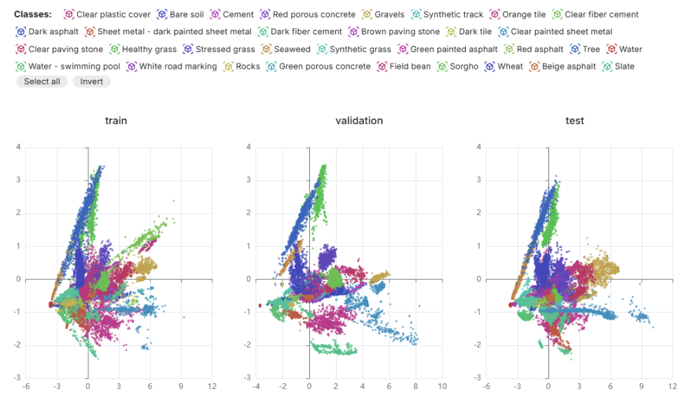\n\nFigure 1: First and second PCA components showing the scores distributions according to classes and subset (train, validation and test) for the Toulouse dataset split #5.\n\n### Original Baseline (RF and self-supervised MAE+RF)\n\nThoreau et al. (2024) first present a RF model trained using the Labeled Training Set to provide a fully supervised baseline. Subsequently, an MAE was pre-trained using the self-supervised masked reconstruction pretext task, a method where the model is forced to reconstruct the full input spectrum given only a subset of spectral channels. This process compels the encoder to learn robust, low-dimensional representations of the data’s intrinsic chemical and material properties from the unmasked regions of the input spectra, leveraging the total available data from the Unlabeled Pool, Labeled Pool, and Labeled Training Set for pre-training. It is worth pointing out that the MAE’s performance relies on the diversity of the spectral data it sees, and the Labeled Pool provides crucial spectral diversity across all classes. Therefore, the labels, while not used directly in the MAE’s reconstruction loss function, are used indirectly to ensure the necessary spectral diversity is present in the data. Finally, the MAE + RF classifier is trained on the MAE embeddings.\n\n### Metaspectral’s Supervised Approach (CNN)\n\nMetaspectral’s Deep Learning CNN was designed for spectral classification and trained end-to-end (feature extraction and classification jointly optimized) under two distinct scenarios:\n\nScenario A: The CNN was trained only on the ~ 13% Labeled Training Set, matching the exact supervised data input used by the paper’s RF model baseline.\n\nScenario B: The CNN was trained on the combined set of the Labeled Training Set and the Labeled Pool, utilizing approximately 42% of the total labeled pixels. This includes some of the information provided to the MAE but does not utilize the spectral data from the Unlabeled Pool.\n\n## Results and Discussion\n\nAll benchmark results are the ones of the test set, presented as averages across all splits (in the paper as well as in the results presented below). As shown in table 1, Metaspectral’s model led to an improvement of the F1 score over both the RF and MAE+RF baselines, demonstrating and validating the efficiency and predictive power of our optimized single-stage deep learning architecture.\n\n| Model | Data Pools | OA | F1 score |\n| --- | --- | --- | --- |\n| RF (paper) | Labeled Training Set | 0.75 | 0.65 |\n| MAE+RF (paper) | Labeled Training Set with MAE pre-trained on all pools | 0.85 | 0.77 |\n| Metaspectral’s CNN (Scenario A) | Labeled Training Set | 0.79 | 0.78 |\n| Metaspectral’s CNN (Scenario B) | Labeled Training Set + Labeled Pool | 0.85 | 0.84 |\n\nTable 1: Averaged test results from the RF, MAE+RF and CNN models trained using different data pools of the Toulouse dataset. OA = Overall Accuracy.\n\nWhen comparing the models, it can be noticed that Metaspectral’s Scenario A CNN achieved an F1 score of 0.78 using only the ~13% Labeled Training Set. This model immediately surpassed the F1 score performance not only of the RF but also of the two-stage MAE+RF pipeline (F1=0.77).\n\nAnother notable observation is that both the MAE+RF baseline and Metaspectral’s CNN in Scenario B achieved the same Overall Accuracy (OA) of 0.85. However, the Metaspectral CNN yielded a significantly higher F1 score (0.84 vs. 0.77). This distinction is important for the Toulouse dataset, which exhibits a long-tailed class distribution. Since OA is dominated by a model’s performance on the majority classes, the superior F1 score (the harmonic mean of precision and recall) confirms that the CNN architecture provides better predictive reliability across all 32 land cover classes, and particularly the minority classes.\n\nFinally, the increase of the F1 score in Metaspectral’s Scenario B of 7% above the RF+MAE baseline model suggests that the most valuable information within the available training data is the high-quality ground-truth label rather than the unlabelled data pool, which the CNN architecture exploits maximally through end-to-end learning. The relative lower F1 score of the MAE+RF pipeline compared to both scenarios could potentially be attributed to two factors. First, while the MAE effectively learned generalized spectral features from the vast UP (contributing to the high OA), these features may not have been optimally disentangled or precise enough to robustly separate the minority, long-tailed classes, which are critical for the F1 score. A structural factor potentially limiting the MAE’s efficacy is the high spectral collinearity inherent in hyperspectral data. Second, the use of an RF classifier in the second stage of the baseline pipeline decouples the feature extraction (MAE) from the final classification task.\n\nThe dataset split #5 is the one that yielded the best model with OA and F1 score both of 0.89. Model results can be visualized on the [Clarity sandbox here](https://clarity.metaspectral.com/models?modelId=2063&tab=overview&modelVersionId=4917). An example of classification inference is given in Figure 2 below and is also available on the [Clarity sandbox for two entire AisaFENIX images](https://clarity.metaspectral.com/spectral-explorer/2674?record=HSI-14283).\n\n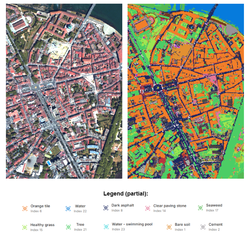\n\nFigure 2: Toulouse’s Saint-Cyprien neighborhood seen in False RGB color (left) and as a pixel-wise land cover classification map obtained from the CNN (right). Only a partial legend of the main classes is provided below and we refer the reader to the Clarity sandbox for an exhaustive legend. \n\n## Conclusions\n\nIn conclusion, Metaspectral’s Deep Learning CNN sets a new performance standard for pixel-wise classification on the Toulouse Hyperspectral Dataset. Our average F1 score of 0.84 is attributable to the architectural strength and efficacy of maximizing high-quality labeled data in a fully supervised training regime.","bodyHtml":"
The Toulouse Hyperspectral Dataset (Thoreau et al., 2024) provides a benchmark for validating pixel-wise classification techniques in challenging, uneven classes and limited-label environments. The dataset, acquired over Toulouse (France), using the airborne AisaFENIX sensor, features a very high spatial resolution (1 m Ground Sampling Distance) and 310 contiguous spectral channels spanning the 400 nm to 2500 nm range. This rich spectral information, combined with a sparse but highly detailed ground truth of 32 land cover classes, makes it ideal for testing model performances and generalization. The original paper’s baseline employed a two-stage approach involving a self-supervised Masked Autoencoder (MAE), to learn spectral representations, followed by a Random Forest (RF) classifier (MAE+RF). It achieved an overall accuracy of 0.85 and an F1 score of 0.77.
\n
Metaspectral is frequently asked about the performance of its Deep Learning (DL) CNN models that were specifically developed for pixel-wise classification, target detection, regression and unmixing tasks on hyperspectral data. Here we sought to demonstrate the efficiency and predictive power of our CNN classifier. We benchmarked our single-stage supervised model against the established MAE+RF pipeline. Our results validate that Metaspectral’s CNN not only maintains competitive performance even with the smallest labeled data subset but also surpasses the original F1 score baseline by a significant margin when trained on all available labeled data. This achievement positions Metaspectral’s model as state-of-the-art for this benchmark. The data and results presented here can be accessed directly on the Clarity sandbox.
\n
Experimental Setup
\n
To ensure robust evaluation, the dataset utilizes 8 spatially disjoint splits. Each split is divided into:
\n
Unlabeled Pool: ~ 2.6 million truly unlabeled pixels. This vast pool was used by the MAE for pre-training. It was not used at all by our CNN.
\n
Labeled Training Set: The small subset used for supervised training of the final classifier in the paper’s baseline (~ 13% of total labeled pixels).
\n
Labeled Pool: An additional, spatially disjoint subset of labeled pixels designated for self-supervised training, active learning, or direct supervised training (accounting for ~ 29% of total labeled pixels).
\n
Test Set: Used for final evaluation (fixed in all experiments).
\n
These splits can be reproduced with the code provided on the TlseHypDataSet GitHub repository. Each split was uploaded on Metaspectral’s Clarity platform to create a corresponding Dataset. Clarity gives an overview of the Dataset through the first and second PCA components (Figure 1) for the train, validation and test subsets. The dataset for split #5 can be visualized on the Clarity sandbox here.
\n
\n
Figure 1: First and second PCA components showing the scores distributions according to classes and subset (train, validation and test) for the Toulouse dataset split #5.
\n
Original Baseline (RF and self-supervised MAE+RF)
\n
Thoreau et al. (2024) first present a RF model trained using the Labeled Training Set to provide a fully supervised baseline. Subsequently, an MAE was pre-trained using the self-supervised masked reconstruction pretext task, a method where the model is forced to reconstruct the full input spectrum given only a subset of spectral channels. This process compels the encoder to learn robust, low-dimensional representations of the data’s intrinsic chemical and material properties from the unmasked regions of the input spectra, leveraging the total available data from the Unlabeled Pool, Labeled Pool, and Labeled Training Set for pre-training. It is worth pointing out that the MAE’s performance relies on the diversity of the spectral data it sees, and the Labeled Pool provides crucial spectral diversity across all classes. Therefore, the labels, while not used directly in the MAE’s reconstruction loss function, are used indirectly to ensure the necessary spectral diversity is present in the data. Finally, the MAE + RF classifier is trained on the MAE embeddings.
\n
Metaspectral’s Supervised Approach (CNN)
\n
Metaspectral’s Deep Learning CNN was designed for spectral classification and trained end-to-end (feature extraction and classification jointly optimized) under two distinct scenarios:
\n
Scenario A: The CNN was trained only on the ~ 13% Labeled Training Set, matching the exact supervised data input used by the paper’s RF model baseline.
\n
Scenario B: The CNN was trained on the combined set of the Labeled Training Set and the Labeled Pool, utilizing approximately 42% of the total labeled pixels. This includes some of the information provided to the MAE but does not utilize the spectral data from the Unlabeled Pool.
\n
Results and Discussion
\n
All benchmark results are the ones of the test set, presented as averages across all splits (in the paper as well as in the results presented below). As shown in table 1, Metaspectral’s model led to an improvement of the F1 score over both the RF and MAE+RF baselines, demonstrating and validating the efficiency and predictive power of our optimized single-stage deep learning architecture.
Labeled Training Set with MAE pre-trained on all pools
0.85
0.77
Metaspectral’s CNN (Scenario A)
Labeled Training Set
0.79
0.78
Metaspectral’s CNN (Scenario B)
Labeled Training Set + Labeled Pool
0.85
0.84
\n
Table 1: Averaged test results from the RF, MAE+RF and CNN models trained using different data pools of the Toulouse dataset. OA = Overall Accuracy.
\n
When comparing the models, it can be noticed that Metaspectral’s Scenario A CNN achieved an F1 score of 0.78 using only the ~13% Labeled Training Set. This model immediately surpassed the F1 score performance not only of the RF but also of the two-stage MAE+RF pipeline (F1=0.77).
\n
Another notable observation is that both the MAE+RF baseline and Metaspectral’s CNN in Scenario B achieved the same Overall Accuracy (OA) of 0.85. However, the Metaspectral CNN yielded a significantly higher F1 score (0.84 vs. 0.77). This distinction is important for the Toulouse dataset, which exhibits a long-tailed class distribution. Since OA is dominated by a model’s performance on the majority classes, the superior F1 score (the harmonic mean of precision and recall) confirms that the CNN architecture provides better predictive reliability across all 32 land cover classes, and particularly the minority classes.
\n
Finally, the increase of the F1 score in Metaspectral’s Scenario B of 7% above the RF+MAE baseline model suggests that the most valuable information within the available training data is the high-quality ground-truth label rather than the unlabelled data pool, which the CNN architecture exploits maximally through end-to-end learning. The relative lower F1 score of the MAE+RF pipeline compared to both scenarios could potentially be attributed to two factors. First, while the MAE effectively learned generalized spectral features from the vast UP (contributing to the high OA), these features may not have been optimally disentangled or precise enough to robustly separate the minority, long-tailed classes, which are critical for the F1 score. A structural factor potentially limiting the MAE’s efficacy is the high spectral collinearity inherent in hyperspectral data. Second, the use of an RF classifier in the second stage of the baseline pipeline decouples the feature extraction (MAE) from the final classification task.
\n
The dataset split #5 is the one that yielded the best model with OA and F1 score both of 0.89. Model results can be visualized on the Clarity sandbox here. An example of classification inference is given in Figure 2 below and is also available on the Clarity sandbox for two entire AisaFENIX images.
\n
\n
Figure 2: Toulouse’s Saint-Cyprien neighborhood seen in False RGB color (left) and as a pixel-wise land cover classification map obtained from the CNN (right). Only a partial legend of the main classes is provided below and we refer the reader to the Clarity sandbox for an exhaustive legend.
\n
Conclusions
\n
In conclusion, Metaspectral’s Deep Learning CNN sets a new performance standard for pixel-wise classification on the Toulouse Hyperspectral Dataset. Our average F1 score of 0.84 is attributable to the architectural strength and efficacy of maximizing high-quality labeled data in a fully supervised training regime.
","updatedAt":"2026-04-23T23:30:39.131Z","createdAt":"2026-04-23T20:30:12.894Z","_status":"published"},{"id":13,"title":"Metaspectral and Armada Partner to Unlock Remote Real-Time AI Analysis of Hyperspectral Imagery","slug":"metaspectral-and-armada-partner-to-unlock-remote-real-time-ai-analysis-of-hyperspectral-imagery","excerpt":"Metaspectral, is partnering with Armada, an edge computing pioneer redefining the future of connectivity, compute, and artificial intelligence (AI).","description":null,"type":"Article","author":{"id":2,"name":"Francis Doumet","slug":"francis-doumet","email":null,"title":null,"bio":null,"updatedAt":"2026-04-23T20:29:55.219Z","createdAt":"2026-04-23T20:29:55.218Z"},"category":null,"heroImage":{"id":147,"alt":"Metaspectral and Armada Partner to Unlock Remote Real-Time AI Analysis of Hyperspectral Imagery","caption":null,"sourcePath":"../src/content/blog/metaspectral-and-armada-partner-to-unlock-remote-real-time-ai-analysis-of-hyperspectral-imagery/metaspectral-and-armada-partner-to-unlock-remote-real-time-ai-analysis-of-hyperspectral-imagery.jpeg","updatedAt":"2026-04-23T23:27:30.230Z","createdAt":"2026-04-23T23:27:30.230Z","url":"/api/media/file/metaspectral-and-armada-partner-to-unlock-remote-real-time-ai-analysis-of-hyperspectral-imagery-1.jpeg","thumbnailURL":"/api/media/file/metaspectral-and-armada-partner-to-unlock-remote-real-time-ai-analysis-of-hyperspectral-imagery-1-320x102.jpg","filename":"metaspectral-and-armada-partner-to-unlock-remote-real-time-ai-analysis-of-hyperspectral-imagery-1.jpeg","mimeType":"image/jpeg","filesize":8225,"width":639,"height":203,"focalX":50,"focalY":50,"sizes":{"thumbnail":{"url":"/api/media/file/metaspectral-and-armada-partner-to-unlock-remote-real-time-ai-analysis-of-hyperspectral-imagery-1-320x102.jpg","width":320,"height":102,"mimeType":"image/jpeg","filesize":4028,"filename":"metaspectral-and-armada-partner-to-unlock-remote-real-time-ai-analysis-of-hyperspectral-imagery-1-320x102.jpg"},"card":{"url":null,"width":null,"height":null,"mimeType":null,"filesize":null,"filename":null}}},"publishedAt":"2024-05-28T07:00:00.000Z","legacySourcePath":"../src/content/blog/metaspectral-and-armada-partner-to-unlock-remote-real-time-ai-analysis-of-hyperspectral-imagery/index.md","bodyMarkdown":"[Metaspectral](https://metaspectral.com/), is partnering with [Armada](https://www.armada.ai/), an edge computing pioneer redefining the future of connectivity, compute, and artificial intelligence (AI).\n\n“Through this partnership, we can bring real-time AI analysis of hyperspectral imagery to remote areas by leveraging Armada’s physical data processing and connectivity infrastructure capabilities,” said Francis Doumet, CEO and co-founder of Metaspectral. “Hyperspectral imagery captured by remote cameras and drones can offer high impact decision-making support with the level of detail it provides.”\n\nHyperspectral images capture much greater detail than traditional cameras, including light from beyond the visible spectrum. This makes it possible to remotely identify the composition, quality, and abundance of materials and gasses using imagery alone.\n\nArmada is collaborating with Starlink to bring high-bandwidth edge computing and satellite internet connectivity to the world’s most remote environments, including oil rigs, mines, and remote combat zones.\n\n“Hyperspectral imagery can be used in the oil and gas sector to detect pipeline leaks, monitor vegetation health, and identify hydrocarbon reservoirs. Similarly, mining companies can use it for mineral identification, prospecting support, and monitoring environmental impacts such as soil erosion, vegetation health, and water quality,” said Migel Tissera, CTO and co-founder of Metaspectral. “Hyperspectral imagery also has extensive military applications, including surveillance, detection, and identification of hidden objects, terrain assessment, and more.”\n\nMetaspectral’s advanced computer vision capabilities will be integrated into Armada’s Edge AI Marketplace, a dynamic hub for AI solutions and applications. Its proprietary data compression algorithms also enable real-time analysis and transmission from satellite and terrestrial sources without compromising image quality.\n\nLed by CEO Dan Wright, Armada offers mobile, self-contained data centers (Galleons) that can be rapidly deployed anywhere to provide real-time data processing, as well as a software platform (Commander), which serves as the single portal for observability and management of all edge operations.\n\n“With Armada’s expertise in AI-powered solutions and Edge Infrastructure, combined with Metaspectral’s cutting-edge computer vision capabilities, we see a tremendous opportunity to help organizations unlock the power of real-time insights and advanced analytics to drive business growth and innovation,” said Uday Tennety, VP of Product Management at Armada. “We look forward to ensuring our joint customers across critical industries are able to glean actionable insights from their data, optimize processes to prioritize agility and precision, and streamline operations.”","bodyHtml":"
Metaspectral, is partnering with Armada, an edge computing pioneer redefining the future of connectivity, compute, and artificial intelligence (AI).
\n
“Through this partnership, we can bring real-time AI analysis of hyperspectral imagery to remote areas by leveraging Armada’s physical data processing and connectivity infrastructure capabilities,” said Francis Doumet, CEO and co-founder of Metaspectral. “Hyperspectral imagery captured by remote cameras and drones can offer high impact decision-making support with the level of detail it provides.”
\n
Hyperspectral images capture much greater detail than traditional cameras, including light from beyond the visible spectrum. This makes it possible to remotely identify the composition, quality, and abundance of materials and gasses using imagery alone.
\n
Armada is collaborating with Starlink to bring high-bandwidth edge computing and satellite internet connectivity to the world’s most remote environments, including oil rigs, mines, and remote combat zones.
\n
“Hyperspectral imagery can be used in the oil and gas sector to detect pipeline leaks, monitor vegetation health, and identify hydrocarbon reservoirs. Similarly, mining companies can use it for mineral identification, prospecting support, and monitoring environmental impacts such as soil erosion, vegetation health, and water quality,” said Migel Tissera, CTO and co-founder of Metaspectral. “Hyperspectral imagery also has extensive military applications, including surveillance, detection, and identification of hidden objects, terrain assessment, and more.”
\n
Metaspectral’s advanced computer vision capabilities will be integrated into Armada’s Edge AI Marketplace, a dynamic hub for AI solutions and applications. Its proprietary data compression algorithms also enable real-time analysis and transmission from satellite and terrestrial sources without compromising image quality.
\n
Led by CEO Dan Wright, Armada offers mobile, self-contained data centers (Galleons) that can be rapidly deployed anywhere to provide real-time data processing, as well as a software platform (Commander), which serves as the single portal for observability and management of all edge operations.
\n
“With Armada’s expertise in AI-powered solutions and Edge Infrastructure, combined with Metaspectral’s cutting-edge computer vision capabilities, we see a tremendous opportunity to help organizations unlock the power of real-time insights and advanced analytics to drive business growth and innovation,” said Uday Tennety, VP of Product Management at Armada. “We look forward to ensuring our joint customers across critical industries are able to glean actionable insights from their data, optimize processes to prioritize agility and precision, and streamline operations.”


